A0. MLC Foundations
Classic control theory defines two types of control systems: Open-Loop Control Systems and Closed-Loop Control Systems. Next a brief definition of both:
- Open-Loop Control Systems: On these systems the output of the system is not compared with the input reference. These systems are calibration based. Examples of these system are the electric pots, a scale, etc. Figure N°1 schematize this model.
 |
|---|
| Figure N°1: Open Loop Control System, being wr a reference signal, b the actuation signal, wd external perturbations, wn noise introduced by sensors and s the output signal |
- Closed-Loop Control Systems: Also known as Feedback Control Systems, on this type of systems an input reference is used as feedback, what generates an error control function. The feedback signal could be an input of the system or function derived from it. The error function is used to specify the actuation to be used as input of the analyzed physical system. Examples of these systems are the ABS brake systems, Thermoregulation, etc. Figure N°2 schematize this model.
 |
|---|
| Figure N°2: Figura N°2: Close-Loop Control System, being wr a reference signal, b the actuation signal, Ɛ an error function, wd external perturbations, wn noise introduced by sensors and s the output signal |
Even though Close-Loop Control Systems are complex and more difficult to maintain that their counterpart, they are the ones which let us stabilize physical systems affected by external disturbances. For this reason the model of this kind of systems are the one used to solve complex problems (non-linear, chaotic, etc.) with a high degree of external variables involved.
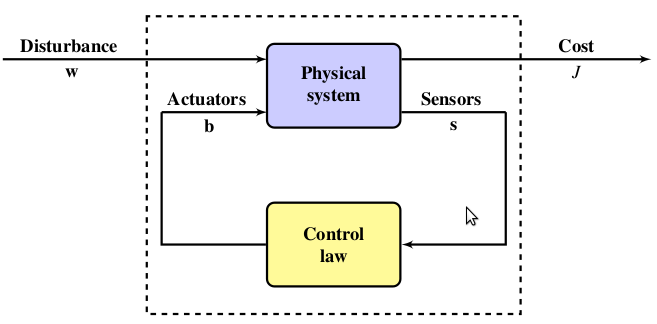
Design a control law to stabilize a particular system could be a challenge. The main reason is that knowing the mathematical model of a system could not be enough because external disturbances must be taken into account. For this reason, it is important to be able to measure the quality of a control law. The Figure N°3 shows a Close-Loop Control System with the addition of a Cost Function. The evaluation of a control law against the Cost Function give as a result the number J. This value must converge to zero when the solution found is optimal. The Cost Function is the tool used by MLC to find optimal control laws. In the following section we will talk how is that MLC use this tool to fulfill its goal.
MLC is a framework that allows the user to discover control rules. MLC framework objective is to automatize the generation of the system control models, that we will refer as "controllers", using as guide the output quality of every generated solution (solutions are generated by the framework itself). Every generated solution is processed using Machine Learning methods, which has been designed to search new controllers inside the a space of valid solutions. Figure N°4 shows a simple representation of the framework architecture.
 |
|---|
| Figure N°3: MLC block diagram |
Figure N° 3 shows how MLC replace the control law of the system. MLC receives as input the s signal and a cost value (J) related to the control law, which is the output of the Cost Function that is evaluated with the output/s of the physical system. With all the input values, MLC generates a new control law with the objective of minimize or maximize the output of the Cost Function.
The Cost Function is the framework element that is defined by the user. It is user responsibility to design and define it for the type of problem to resolve (i.e. it's related with the Physical system). For example, in a turbulent flow stabilization system we can consider that the system converge if the velocity of the different points in the system are similar (this would mean that the system becomes laminar). In this example, a valid cost function would be the one that tends to zero when the speeds of the flow particles are homogeneous.
The following section will give the user an introduction on the Machine Learning techniques used by MLC to find new control laws. The user must take into consideration that the control laws are named as Individuals inside MLC due to the use of Machine Learning and Genetic Programming jargon inside the tool.
Machine Learning is a subfield of the computer sciences based in Pattern Recognition and Computational Learning Theory. This science is commonly used to identify systems inside of a high dimensional search space using learning techniques. There are lots of learning techniques that could be applied in the Machine Learning field (Gradient search and Monte-Carlo Statistical Analysis to name two examples). All these techniques has as main common characteristic the generation of suboptimal solutions or associated with a high cost when the search space is too big. Is at this point where Genetic Programming has a key role due to they are optimal to resolve this type of problems.
Genetic Programming and Genetics Algorithms are based in the individual generations propagation, also know as populations. These individuals are selected in function of the results of the Cost/Fitness Function (J) evaluation. The result of these function is referred as cost or fitness. Figure N°4 shows a detailed diagram that explains the application of this functions on MLC Framework. In the figure, the b = K(s) individual is evaluated in the dynamic system. From this evaluation is obtained the fitness value of the individual. Once all the populations has been evaluated, MLC generates a new population using different techniques of Genetics Programming.
 |
|---|
| Figure N°4: MLC general workflow |
In MLC an individual is represented as a conjunction of maths functions and parameters with a recursive function tree structure. The framework allows the use of the maths functions of: sum, subtraction, multiplication and division. It is also possible to extend the range adding function like exponential, sine, hyperbolic tangent just to name a few. As it was previously mention, the individual is stored in a tree structure model. The no-leaf nodes of the tree stores constants or system parameters (experiment sensors are the most common use) while the leaf nodes stores the mathematics functions. Figure N°5 shows the MLC individual model. The tree structure representation of the individuals is ideal for the genetics algorithms that MLC uses.
 |
|---|
| Figure N°5: Individual Tree |
Usually, the first Individual generation is randomly generated using the available functions for the experiment (i.e. constants, maths functions and sensor variables). Constants range and maths functions that can be used as individual components are part of the experiment configuration that the user must set up. Once the first individual generation (Population) is generated, MLC starts the evaluation process of the Population. The evaluation consists in taking measures from the configured sensors of the experiment and using the readings in the individual that is being evaluated (remember that a part of the Individual could be a sensor variable). These evaluations generates the fitness value of the Individual. Once all the Individuals of the Population has been evaluated, MLC begins with the evolution process of the Population. The Figure N°6 shows how the algorithms works. And explanation of them is given below:
-
Elitism: This algorithm takes care to choose the best individuals from the population in order to be part of the next generation (i.e. choose individuals that "survives" to the next population)
-
Replication: With a random behaviour, some individuals from the current population are selected and are allowed to be part of the next generation.
-
Crossover: Individuals with similar fitness value have a random components exchange (no leaf nodes are exchanged between individuals), generating a new individual. This new individual will be part of the next generation.
-
Mutation: Some parts of the individuals are randomly modified and are allowed to be part of the next generation.
 |
|---|
| Figure N°6: MLC evolution techniques |
When the Population evolution process is done, MLC executes a new evaluation of the Population. From this moment on, the evaluation-evolution process is repeated until a break point is reached. Usually, MLC uses as a break point a number of generations to be evaluated and evolved that is selected by the user. Figure N°7 shows a flow diagram of the process involved in the generation of new Populations.
 |
|---|
| Figure N°7: MLC workflow |