This is my fork of PGND (Particle-Grid Neural Dynamics), extended with three model variants that progressively add visual supervision and camera conditioning on top of the baseline.
The goal: take a state-of-the-art learned cloth dynamics method, get it running on data I collected from my own robot, and then extend it — first with a differentiable render loss during training, then with live camera conditioning at rollout time.
Image below is from the original PGND authors and shows their benchmark setup, not my hardware or results.

PGND learns deformable object dynamics from RGB-D video using a particle-grid hybrid representation. The baseline model predicts cloth state purely from geometry (particle positions and velocities), autoregressively rolling out future states from an initial condition.
My experiments use this as the starting point, adding visual signals at two stages: during training (render loss) and at rollout time (camera conditioning).
Standard PGND training on my cloth dataset. Supervises on particle position loss (loss_x, MSE per step) only — no visual signal, no camera input. Predicts cloth dynamics purely from geometric state.
pgnd-comparison-all.mp4
Key files: experiments/train/train_eval.py, experiments/train/eval.py
Adds a differentiable render loss on top of the baseline to penalise predictions that are geometrically plausible but visually wrong.
What it does:
- A frozen
diff-gaussian-rasterizerprojects predicted particle state into camera space - Rendered frames are compared against ground truth RGB using two losses:
λ_render = 0.1— DINOv2 feature distance (semantic similarity)λ_ssim = 0.2— SSIM (structural similarity)
- The render loss gradient flows back through the rasterizer into the dynamics model
Why this matters: The position loss (MSE on particles) can be satisfied by predictions that look wrong visually — cloth bunched in the wrong place, wrong fold direction, etc. The render loss adds a signal that's sensitive to visual appearance, not just particle distance.
Key files: experiments/train/render_loss.py, experiments/train/train_eval_render_loss.py
pgnd-ep0201-baseline.mp4
Takes the render loss further and adds camera conditioning at rollout time, so the model can see when its predictions have drifted from reality.
Two changes on top of Phase 2:
-
Mesh-constrained Gaussian Splatting — instead of using LBS (linear blend skinning) to approximate how Gaussians deform with the particle mesh, each Gaussian is bound directly to a face of the particle mesh and deforms with it exactly. This removes an approximation error that limited how sharp the render loss gradient could be in Phase 2.
-
Camera conditioning at rollout — a frozen DINOv2 backbone encodes the current camera observation at each rollout step. This feature is injected into the dynamics model as an additional input, giving it a correction signal: if predicted state drifts from what the cameras see, the model can self-correct rather than compounding the error.
Key files:
experiments/train/pgnd_visual.py— visual PGND model definitionexperiments/train/mesh_gaussian_model.py— mesh-constrained Gaussian representationexperiments/train/visual_encoder.py— DINOv2 feature encoder for camera conditioningexperiments/train/train_eval_visual.py— training loop for visual PGNDexperiments/train/anchor_gaussians_to_mesh.py— binds Gaussians to mesh faces
pgnd-ep0201-phase2.mp4
All three models are evaluated on held-out episodes, rolling out 30 steps autoregressively from ground truth initial conditions. Three metrics:
- MDE (Mean Displacement Error) — average per-particle Euclidean distance to ground truth. Sensitive to individual particle drift.
- Chamfer Distance — bidirectional nearest-neighbour distance between predicted and GT point clouds. Penalises large-scale shape mismatch without requiring correspondence.
- EMD (Earth Mover's Distance) — minimum transport cost to match predicted to GT distribution. More sensitive to global deformation failure modes than Chamfer.
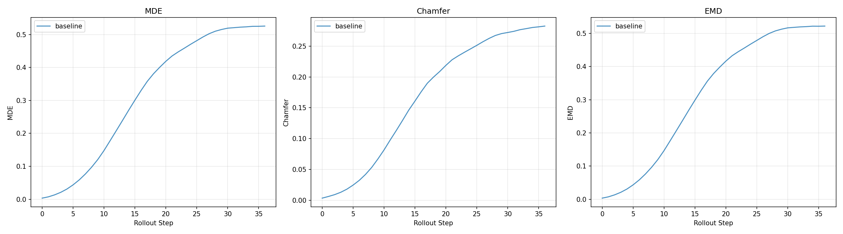
Prediction error over 30 rollout steps. Lower is better; all metrics grow with rollout horizon as errors compound.
The same held-out cloth manipulation rollout predicted by each model:
| Model | Video |
|---|---|
| Baseline (100k) — geometry only | video |
| Phase 2 (40k) — + DINOv2 render loss + SSIM | video |
| Visual PGND (70k) — + mesh GS + camera conditioning | video |
pgnd-ep0201-visual.mp4
All episodes — baseline vs. visual PGND
Full writeup: tabithako.github.io/projects/cloth-dynamics
experiments/train/convert_pgnd_to_phystwin.py— converts PGND episode format to PhysTwin for cross-pipeline comparisonexperiments/train/test_phystwin_generalization.py— evaluates how well PhysTwin-fitted parameters generalise to novel PGND episodes
experiments/train/compare_3_ablations.py/compare_ablations.py/compare_phase2.py— side-by-side rollout comparisons across model variantsexperiments/train/generate_eval_videos.py— batch video generation for the full held-out eval setexperiments/train/viz_phase2.py— Phase 2 render loss visualisation
episode_matches.json— maps PGND episode IDs to corresponding PhysTwin trajectory recordings for cross-pipeline evaluation
The perception pipeline is where the real work is. Getting CoTracker running reliably on my specific cameras, lighting, and occlusion patterns required more iteration than training the dynamics model. Data quality limits everything downstream.
Visual conditioning helps but training is fragile. DINOv2 features add useful signal, but the render loss curriculum schedule matters a lot. Phase 2 is the most stable improvement; Visual PGND at 70k is still training.
Evaluation set size matters. A 5-episode eval showed a 20% improvement. A 40-episode eval showed ~1%. The 40-episode numbers are the ones I use.
Learning Particle Dynamics for Manipulating Rigid Bodies, Deformable Objects, and Fluids Yunzhu Li et al. — project page