Probablistic Algorithm for TCP/UDP Packet Flow Analysis

Implementation of algorithms for packet flow analysis (limited to TCP and UDP flows). Contains two variants of a program to compute the packet count:

1. Exact count without dealing with space complexity
2. Optimized implementation returning an approximate count (within a specific bound) using a probablistic algorithm/data structure (count-min sketch)

Directory Layout

.
|-- data ... Contains packet dumps for offline analysis
|   |-- http.cap
|   |-- lbl.pcap
|   `-- mb.pcap
|
|-- helper ... Helper functions used during development
|   
|-- plots ... Plots of frequency distributions of packet flows
|   
|-- TaskOne ... Variant One (using a simple hash table to compute exact count)
|   |-- a.out
|   |-- HIST_FILE.txt ... Stores frequencies of unique flow tuples
|   |-- packet_analysis.cc
|   |-- packet_analysis.h
|   |-- plot_hist.py ... Generates frequency distribution plots from HIST_FILE
|   `-- profiling ... Valgrind massif memory profiling
|
`-- TaskTwo ... Variant Two (optimized using a count-min sketch, returns approximate count within bounds)
    |-- a.out
    |-- count_min_sketch.cc
    |-- count_min_sketch.h
    |-- FLOW_FILE.txt
    |-- packet_analysis.cc
    |-- packet_analysis.h
    `-- profiling ... Stores the unique flow tuples (generated from TaskOne)

Basic Usage

Note: Significance of generated files is specified in the directory layout section

1. Compile and run the TaskOne/packet_analysis.cc

g++ packet_analysis.cc -lpcap
./a.out [NAME OF DATA FILE]

2. This will generate HIST_FILE.txt and FLOW_FILE.txt (in the TaskTwo directory)
3. Compile and run the TaskTwo/packet_analysis.cc

g++ packet_analysis.cc count_min_sketch.cc -lpcap
./a.out [NAME OF DATA FILE]

4. This will generate the count-min sketch (by analyzing packets from the input data file), and then estimate the frequency by reading in unique tuples from FLOW_FILE (generated in TaskOne to avoid having to manually enter flow tuples during the estimation phase).

Advanced Usage (Profiling)

1. To profile the memory usage (heap) of the two variants using Valgrind

valgrind --tool=massif ./a.out [NAME OF DATA FILE]

2. This will generate a massif.out.pid file, which can be analyzed using ms_print

ms_print massif.out.pid file

3. To only display the graph of number of instructions VS memory usage

ms_print massif.out.pid | head -n 35

Results

The following are preliminary results when the two variants are tested using a sample packet dump file (LBL dataset)

Vanilla Hash Map (First Variant)

Valgrind Massif Generated Graph

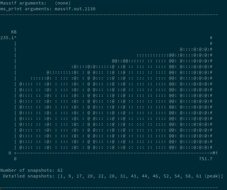
As evident, the hash map has a larger memory footprint (which increases during execution)

Sample of flow counts in the hash map (Pretty Printed)

Flow: (128.3.44.112,1582,148.184.171.6,445) Count: 1
Flow: (218.165.163.184,80,128.3.47.183,4353) Count: 3
Flow: (218.131.115.53,80,128.3.45.128,62337) Count: 5
Flow: (128.3.99.118,993,128.3.44.98,4591) Count: 123
Flow: (218.131.115.53,80,128.3.45.128,62336) Count: 5
Flow: (128.3.45.128,62336,218.131.115.53,80) Count: 5
Flow: (208.233.189.150,80,128.3.45.128,62335) Count: 5
Flow: (128.3.45.128,62335,208.233.189.150,80) Count: 5
Flow: (128.3.45.128,62334,208.233.189.150,80) Count: 5

Count Min Sketch (Second Variant)

Valgrind Massif Generated Graph

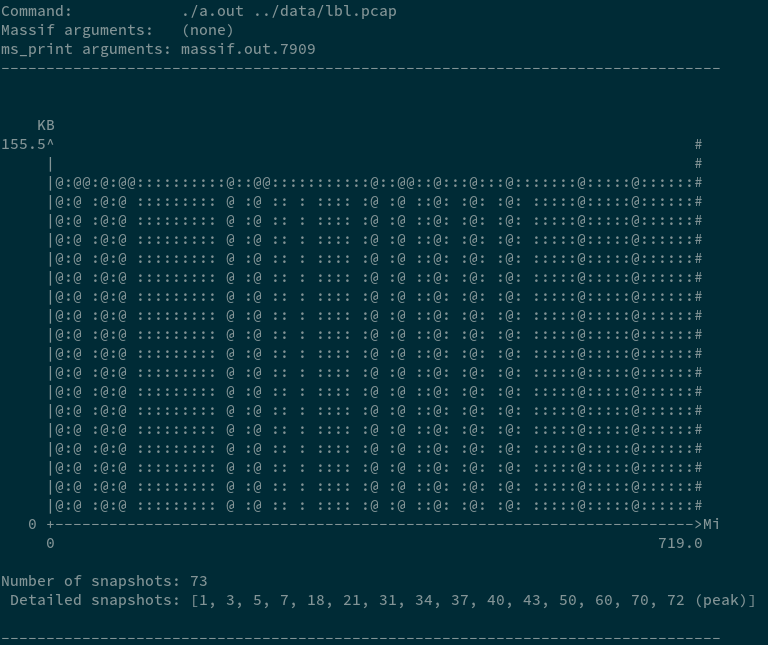
Whereas, the count-min sketch has a constant memory footprint (~150 kB). The difference should be increasingly evident for larger packet dumps with more unique flows.

Sample of flow counts in count-min sketch (Pretty Printed)

Flow: (128.3.44.112,1582,148.184.171.6,445) Estimate: 1
Flow: (218.165.163.184,80,128.3.47.183,4353) Estimate: 10
Flow: (218.131.115.53,80,128.3.45.128,62337) Estimate: 7
Flow: (128.3.99.118,993,128.3.44.98,4591) Estimate: 123
Flow: (218.131.115.53,80,128.3.45.128,62336) Estimate: 5
Flow: (128.3.45.128,62336,218.131.115.53,80) Estimate: 23
Flow: (208.233.189.150,80,128.3.45.128,62335) Estimate: 8
Flow: (128.3.45.128,62335,208.233.189.150,80) Estimate: 5
Flow: (128.3.45.128,62334,208.233.189.150,80) Estimate: 16

Future Work

1. Generate a frequency distribution plot for flow counts using HIST_FILE

python hist_plot.py

2. Depending on the degree of skewness, choose which algorithm to run (either CMS or similar algorithm such as Fast-AGMS). CMS has been observed to have better performance in skewed distributions, whereas Fast-AGMS is better for non-skewed distributions
3. Generating frequency distribution for the sample datasets in the repository results in the following plots

lbl.pcap Flow Frequency Distribution

http.pcap Flow Frequency Distribution

mb.pcap Flow Frequency Distribution

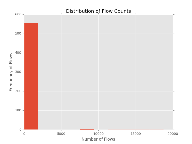
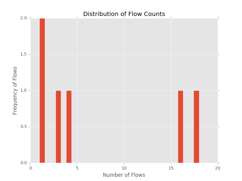
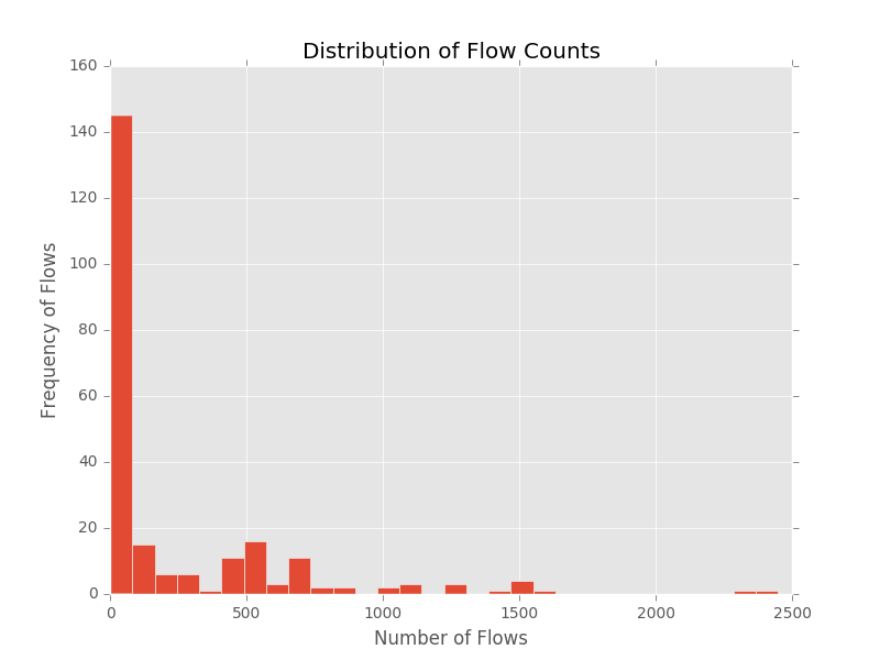
These preliminary plots suggest that CMS is well suited for these datasets.

Note: Need to find datasets with non-skewed flow frequency distributions, to test results.

References

• http://dimacs.rutgers.edu/~graham/pubs/papers/cm-full.pdf
• https://en.wikipedia.org/wiki/Count%E2%80%93min_sketch#cite_note-goyal-5
• http://web.stanford.edu/class/cs168/l/l2.pdf
• http://webdocs.cs.ualberta.ca/~drafiei/papers/cmm.pdf