A comprehensive reference guide covering all essential mathematical formulas used in Data Science and Machine Learning

- Linear Algebra
- Calculus
- Probability
- Statistics
- Linear & Logistic Regression
- Neural Networks
- Optimization Algorithms
- Evaluation Metrics
- Clustering
- Deep Learning
- Dimensionality Reduction
- Information Theory
- Support Vector Machines
- Decision Trees & Ensembles
- Bias-Variance Tradeoff
| Formula | Expression |
|---|---|
| Dot Product | a · b = Σ(aᵢbᵢ) = a₁b₁ + a₂b₂ + ... + aₙbₙ |
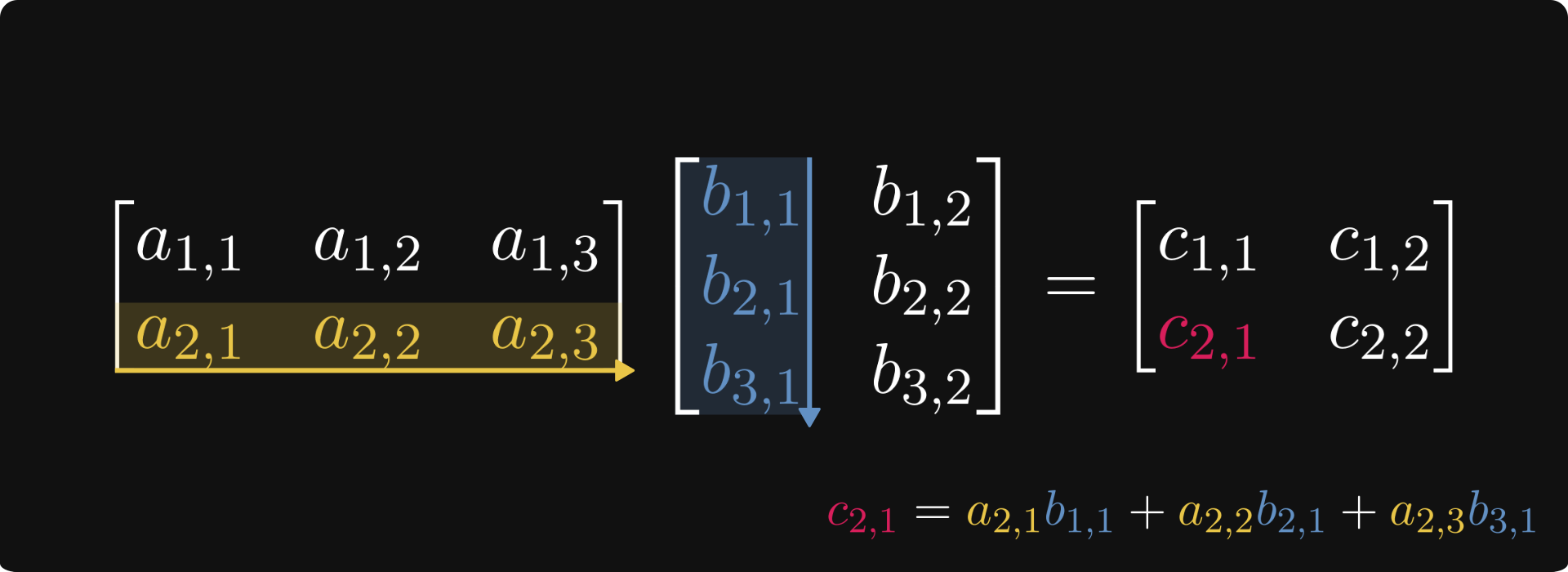
| Matrix Multiplication | C = AB where Cᵢⱼ = Σₖ(AᵢₖBₖⱼ) |
| Transpose | (AB)ᵀ = BᵀAᵀ |
| Identity Matrix | AI = IA = A |
| Inverse Matrix | AA⁻¹ = A⁻¹A = I |
| Norm Type | Formula |
|---|---|
| L1 Norm (Manhattan) | ‖x‖₁ = Σ|xᵢ| |
| L2 Norm (Euclidean) | ‖x‖₂ = √(Σxᵢ²) |
| Frobenius Norm | ‖A‖F = √(ΣᵢΣⱼ aᵢⱼ²) |
Eigenvalue Equation:     Av = λv
Characteristic Equation: det(A - λI) = 0
Trace:                   tr(A) = Σλᵢ = Σaᵢᵢ
Determinant:             det(A) = Πλᵢ
| Rule | Formula |
|---|---|
| Power Rule | d/dx(xⁿ) = nxⁿ⁻¹ |
| Chain Rule | d/dx[f(g(x))] = f'(g(x)) · g'(x) |
| Product Rule | d/dx[f(x)g(x)] = f'(x)g(x) + f(x)g'(x) |
| Quotient Rule | d/dx[f(x)/g(x)] = [f'(x)g(x) - f(x)g'(x)]/g(x)² |
Gradient:        ∇f = [∂f/∂x₁, ∂f/∂x₂, ..., ∂f/∂xₙ]
Hessian Matrix:  Hᵢⱼ = ∂²f/(∂xᵢ∂xⱼ)
Jacobian Matrix: Jᵢⱼ = ∂fᵢ/∂xⱼ
| Function | Derivative |
|---|---|
| Sigmoid | σ'(x) = σ(x)(1 - σ(x)) |
| Tanh | tanh'(x) = 1 - tanh²(x) |
| ReLU | ReLU'(x) = {1 if x > 0, 0 otherwise} |
| Exponential | d/dx(eˣ) = eˣ |
| Logarithm | d/dx(ln x) = 1/x |
Probability:              P(A) = (Favorable outcomes)/(Total outcomes)
Complement Rule:          P(Aᶜ) = 1 - P(A)
Addition Rule:            P(A ∪ B) = P(A) + P(B) - P(A ∩ B)
Multiplication Rule:      P(A ∩ B) = P(A|B)P(B) = P(B|A)P(A)
Conditional Probability:  P(A|B) = P(A ∩ B)/P(B)
Bayes' Rule:      P(A|B) = [P(B|A)P(A)]/P(B)

Extended Form:    P(A|B) = [P(B|A)P(A)]/[P(B|A)P(A) + P(B|Aᶜ)P(Aᶜ)]
💡 Key Application: Fundamental in ML for classification, spam detection, and probabilistic reasoning
| Concept | Formula |
|---|---|
| Expected Value | E[X] = Σ xᵢP(xᵢ) or ∫ xf(x)dx |
| Variance | Var(X) = E[(X - μ)²] = E[X²] - (E[X])² |
| Standard Deviation | σ = √Var(X) |
| Covariance | Cov(X,Y) = E[(X - μₓ)(Y - μᵧ)] |
| Correlation | ρ(X,Y) = Cov(X,Y)/(σₓσᵧ) |
| Measure | Formula |
|---|---|
| Mean | μ = (1/n)Σxᵢ |
| Sample Variance | s² = [1/(n-1)]Σ(xᵢ - x̄)² |
| Population Variance | σ² = (1/n)Σ(xᵢ - μ)² |
| Standard Error | SE = σ/√n |
Z-score:             z = (x - μ)/σ
T-statistic:         t = (x̄ - μ)/(s/√n)
Confidence Interval: CI = x̄ ± z(α/2) · SE
Key Terms:
- Type I Error (α): Rejecting true null hypothesis
- Type II Error (β): Failing to reject false null hypothesis
- Power: 1 - β
| Component | Formula |
|---|---|
| Simple Model | y = β₀ + β₁x + ε |
| Matrix Form | y = Xβ + ε |
| Normal Equation | β = (XᵀX)⁻¹Xᵀy |
| Predicted Values | ŷ = Xβ |
Mean Squared Error (MSE):     MSE = (1/n)Σ(yᵢ - ŷᵢ)²
Root Mean Squared Error:      RMSE = √MSE
Mean Absolute Error (MAE):    MAE = (1/n)Σ|yᵢ - ŷᵢ|
R-squared:                    R² = 1 - [Σ(yᵢ - ŷᵢ)²]/[Σ(yᵢ - ȳ)²]
Adjusted R²:                  R²adj = 1 - [(1 - R²)(n - 1)]/(n - p - 1)
| Component | Formula |
|---|---|
| Sigmoid Function | σ(z) = 1/(1 + e⁻ᶻ) |
| Logit | z = β₀ + β₁x₁ + β₂x₂ + ... + βₙxₙ |
| Probability | P(y=1|x) = σ(wᵀx + b) |
| Odds | Odds = P(y=1)/P(y=0) = eᶻ |
| Log-Odds | log(Odds) = z |
Log Loss (Binary Cross-Entropy):
L = -(1/n)Σ[yᵢlog(ŷᵢ) + (1-yᵢ)log(1-ŷᵢ)]
| Type | Cost Function |
|---|---|
| Ridge (L2) | J(β) = Σ(yᵢ - ŷᵢ)² + λΣβⱼ² |
| Lasso (L1) | J(β) = Σ(yᵢ - ŷᵢ)² + λΣ|βⱼ| |
| Elastic Net | J(β) = Σ(yᵢ - ŷᵢ)² + λ₁Σ|βⱼ| + λ₂Σβⱼ² |
| Function | Formula |
|---|---|
| Sigmoid | σ(x) = 1/(1 + e⁻ˣ) |
| Tanh | tanh(x) = (eˣ - e⁻ˣ)/(eˣ + e⁻ˣ) |
| ReLU | ReLU(x) = max(0, x) |
| Leaky ReLU | f(x) = {x if x > 0, αx otherwise} |
| Softmax | softmax(xᵢ) = eˣⁱ/Σⱼeˣʲ |
Linear Combination:  z⁽ˡ⁾ = W⁽ˡ⁾a⁽ˡ⁻¹⁾ + b⁽ˡ⁾
Activation:          a⁽ˡ⁾ = g(z⁽ˡ⁾)
Output Layer Error:   δ⁽ᴸ⁾ = (a⁽ᴸ⁾ - y) ⊙ g'(z⁽ᴸ⁾)
Hidden Layer Error:   δ⁽ˡ⁾ = [(W⁽ˡ⁺¹⁾)ᵀδ⁽ˡ⁺¹⁾] ⊙ g'(z⁽ˡ⁾)
Weight Gradient:      ∂L/∂W⁽ˡ⁾ = δ⁽ˡ⁾(a⁽ˡ⁻¹⁾)ᵀ
Bias Gradient:        ∂L/∂b⁽ˡ⁾ = δ⁽ˡ⁾
| Variant | Update Rule |
|---|---|
| Batch GD | θ := θ - α∇J(θ) |
| Stochastic GD | θ := θ - α∇J(θ; xⁱ, yⁱ) |
| Mini-batch GD | Uses small batches of data |
Momentum:
  v := βv + (1-β)∇J(θ)
  θ := θ - αv

RMSprop:
  s := βs + (1-β)(∇J)²
  θ := θ - α∇J/√(s + ε)

Adam:
  m := β₁m + (1-β₁)∇J
  v := β₂v + (1-β₂)(∇J)²
  θ := θ - α·m̂/√(v̂ + ε)
| Metric | Formula |
|---|---|
| Accuracy | (TP + TN)/(TP + TN + FP + FN) |
| Precision | TP/(TP + FP) |
| Recall (Sensitivity) | TP/(TP + FN) |
| Specificity | TN/(TN + FP) |
| F1-Score | 2·(Precision·Recall)/(Precision + Recall) |
| F-beta Score | (1 + β²)·(Precision·Recall)/(β²·Precision + Recall) |
                    Predicted
                 Positive  Negative
Actual Positive     TP        FN
       Negative     FP        TN
Legend:
- TP = True Positive
- TN = True Negative
- FP = False Positive (Type I Error)
- FN = False Negative (Type II Error)
TPR (True Positive Rate):  TP/(TP + FN)
FPR (False Positive Rate): FP/(FP + TN)
AUC (Area Under Curve):    ∫₀¹ TPR(FPR⁻¹(x))dx
Objective Function:  minimize Σᵏⱼ₌₁ Σₓ∈Cⱼ ||x - μⱼ||²
Centroid Update:     μⱼ = (1/|Cⱼ|)Σₓ∈Cⱼ x
| Metric | Formula |
|---|---|
| Euclidean | d(x, y) = √(Σᵢ(xᵢ - yᵢ)²) |
| Manhattan | d(x, y) = Σᵢ|xᵢ - yᵢ| |
| Cosine Similarity | cos(θ) = (x·y)/(‖x‖·‖y‖) |
s(i) = [b(i) - a(i)]/max{a(i), b(i)}

Where:
  a(i) = mean distance to points in same cluster
  b(i) = mean distance to points in nearest cluster
Normalize:        x̂ = (x - μ_B)/√(σ²_B + ε)
Scale and Shift:  y = γx̂ + β
Convolution Operation:  (f * g)(t) = Σₓ f(x)g(t - x)
Output Size:            O = [(W - K + 2P)/S] + 1

Where:
  W = input size
  K = kernel size
  P = padding
  S = stride
Hidden State:  hₜ = tanh(Wₓₕxₜ + Wₕₕhₜ₋₁ + bₕ)
Output:        yₜ = Wₕᵧhₜ + bᵧ
Forget Gate:  fₜ = σ(Wf·[hₜ₋₁, xₜ] + bf)
Input Gate:   iₜ = σ(Wᵢ·[hₜ₋₁, xₜ] + bᵢ)
Output Gate:  oₜ = σ(Wo·[hₜ₋₁, xₜ] + bo)
Cell State:   Cₜ = fₜ ⊙ Cₜ₋₁ + iₜ ⊙ C̃ₜ
Training:  Output = mask ⊙ activation / (1 - p)
Testing:   Use all neurons (no dropout)
Covariance Matrix:          Σ = (1/n)XᵀX
Principal Components:       Eigenvectors of Σ
Explained Variance Ratio:   λᵢ/Σⱼλⱼ
Projection:                 Z = XW (W = eigenvectors)
Decomposition:   X = UΣVᵀ
Reduced Form:    X ≈ UₖΣₖVₖᵀ
| Measure | Formula |
|---|---|
| Entropy | H(X) = -Σ P(xᵢ)log₂P(xᵢ) |
| Cross-Entropy | H(p,q) = -Σ p(x)log q(x) |
| KL Divergence | DKL(P‖Q) = Σ P(x)log[P(x)/Q(x)] |
| Mutual Information | I(X;Y) = H(X) - H(X|Y) = H(Y) - H(Y|X) |
| Conditional Entropy | H(Y|X) = -ΣₓΣᵧ P(x,y)log P(y|x) |
Decision Function:  f(x) = wᵀx + b
Margin:             2/||w||
Optimization:       minimize ½||w||²
                    subject to yᵢ(wᵀxᵢ + b) ≥ 1
Objective:   minimize ½||w||² + CΣξᵢ
Constraint:  yᵢ(wᵀxᵢ + b) ≥ 1 - ξᵢ, ξᵢ ≥ 0
| Kernel | Formula |
|---|---|
| Linear | K(x, x') = xᵀx' |
| Polynomial | K(x, x') = (xᵀx' + c)ᵈ |
| RBF (Gaussian) | K(x, x') = exp(-γ‖x - x'‖²) |
| Sigmoid | K(x, x') = tanh(αxᵀx' + c) |
| Measure | Formula |
|---|---|
| Gini Impurity | Gini = 1 - Σᵢ pᵢ² |
| Entropy | H = -Σᵢ pᵢlog₂(pᵢ) |
| Classification Error | E = 1 - max(pᵢ) |
Information Gain: IG(D, A) = H(D) - Σᵥ[(|Dᵥ|/|D|)·H(Dᵥ)]
Bagging (Random Forest):
  Prediction: ŷ = (1/B)Σᵇ fᵇ(x)

AdaBoost:
  Sample Weight:  wᵢ⁽ᵗ⁺¹⁾ = wᵢ⁽ᵗ⁾·exp[αₜ·I(yᵢ ≠ hₜ(xᵢ))]
  Model Weight:   αₜ = ½ln[(1 - εₜ)/εₜ]

Gradient Boosting:
  Update:   Fₘ(x) = Fₘ₋₁(x) + γₘhₘ(x)
  Residual: rᵢₘ = -[∂L(yᵢ, F(xᵢ))/∂F(xᵢ)]
Total Error = Bias² + Variance + Irreducible Error

Bias:     Bias = E[ŷ] - y
Variance: Variance = E[(ŷ - E[ŷ])²]
Key Insights:
- High Bias → Underfitting (model too simple)
- High Variance → Overfitting (model too complex)
- Goal: Find the optimal balance between bias and variance
| Loss | Formula | Use Case |
|---|---|---|
| MSE | L = (1/n)Σ(yᵢ - ŷᵢ)² |
Standard regression |
| MAE | L = (1/n)Σ|yᵢ - ŷᵢ| |
Robust to outliers |
| Huber | L = {½(y - ŷ)² if |y - ŷ| ≤ δ, δ|y - ŷ| - ½δ² otherwise} |
Combines MSE & MAE |
| Loss | Formula | Use Case |
|---|---|---|
| Binary Cross-Entropy | L = -[ylog(ŷ) + (1-y)log(1-ŷ)] |
Binary classification |
| Categorical Cross-Entropy | L = -Σᵢ yᵢlog(ŷᵢ) |
Multi-class classification |
| Hinge Loss | L = max(0, 1 - y·ŷ) |
SVM classification |
| Method | Formula | Range |
|---|---|---|
| Min-Max Scaling | x' = (x - min)/(max - min) |
[0, 1] |
| Z-Score Normalization | x' = (x - μ)/σ |
~ [-3, 3] |
| Max Abs Scaling | x' = x/|max| |
[-1, 1] |
Degree 2: [x₁, x₂] → [1, x₁, x₂, x₁², x₁x₂, x₂²]
Degree 3: [x₁, x₂] → [1, x₁, x₂, x₁², x₁x₂, x₂², x₁³, x₁²x₂, x₁x₂², x₂³]
Contributions are welcome! If you find any errors or want to add more formulas:
- Fork the repository
- Create a new branch (
git checkout -b feature/new-formulas) - Make your changes
- Commit your changes (
git commit -am 'Add new formulas') - Push to the branch (
git push origin feature/new-formulas) - Create a Pull Request
- Mathematics for Machine Learning Book
- Deep Learning Book
- Pattern Recognition and Machine Learning
- Scikit-learn Documentation
- TensorFlow Documentation
- PyTorch Documentation
- Khan Academy - Linear Algebra - Comprehensive free course on vectors, matrices, and transformations
- Khan Academy - Multivariable Calculus - Free course covering derivatives, integrals in multiple dimensions
- Khan Academy - Statistics & Probability - Foundation in probability, random variables, and statistical inference
- 3Blue1Brown - Essence of Linear Algebra - Visual, intuitive video series on linear algebra concepts
- 3Blue1Brown - Essence of Calculus - Beautiful visual explanations of calculus fundamentals
- MIT OCW - Linear Algebra (18.06) - Prof. Gilbert Strang's legendary MIT course
- MIT OCW - Single Variable Calculus - Complete calculus course with problem sets
- MIT OCW - Multivariable Calculus - Extends calculus to multiple variables
- MIT OCW - Matrix Methods in Data Analysis - Linear algebra for ML applications
- StatQuest with Josh Starmer - Clear explanations of statistics and ML concepts
- Coursera - Mathematics for Machine Learning Specialization - Free to audit, covers linear algebra, calculus, and PCA
- Coursera - Data Science Math Skills - Free to audit, basics for data science
- NPTEL - Essential Mathematics for Machine Learning - Indian university course on ML math
- NPTEL - Probability and Statistics - Comprehensive probability course
- CMU Open Learning - Probability & Statistics - Self-paced interactive course
- Immersive Linear Algebra - Interactive linear algebra textbook with visualizations
- Linear Algebra Done Right - Free online version of the popular textbook
- Introduction to Probability - Harvard's Stat 110 course materials
- Think Stats - Free book on probability and statistics for programmers
- Seeing Theory - Visual introduction to probability and statistics
- Statistics Done Wrong - Learn common statistical mistakes to avoid
- Awesome Data Science - Comprehensive open-source Data Science repository to learn and apply towards solving real-world problems
- Awesome Machine Learning - Curated list of awesome ML frameworks, libraries and software (by language)
- Data Science For Beginners by Microsoft - 10-week, 20-lesson curriculum with quizzes and hands-on projects
- ML For Beginners by Microsoft - 12-week, 26-lesson curriculum for Machine Learning beginners
- Python Data Science Handbook - Full text in Jupyter Notebooks covering NumPy, Pandas, Matplotlib, Scikit-Learn
- Data Science Masters - Open-source curriculum for aspiring data scientists
- OSSU Data Science - Path to free self-taught education in Data Science
- Homemade Machine Learning - Python implementations of ML algorithms with math explanations
- ML YouTube Courses - Curated index of quality ML courses on YouTube from Stanford, MIT, Caltech
- Applied ML - Papers and tech blogs on real-world ML applications in production
- Awesome Production ML - Libraries to deploy, monitor, version, scale and secure ML models
- DS Cheatsheets - Collection of Data Science cheatsheets from Python to Big Data
- Free Data Science Books - List of free books for Data Science and Big Data concepts
- Data Science Learning Resources - Curated collection of data science and ML resources
This project is licensed under the MIT License - see the LICENSE file for details.
- Bookmark this page for quick reference during ML projects
- Print specific sections you use frequently
- Practice implementing these formulas in code
- Understand the intuition behind each formula, not just memorization
- Share with fellow ML practitioners and students
Created with ❤️ for the Machine Learning community. Special thanks to all contributors and the open-source ML community.
If you find this helpful, please consider giving it a star! It helps others discover this resource.

Creator & Maintainer
We welcome contributions! If you have:
- Formula corrections or additions
- Documentation improvements
- Feature suggestions
- Bug reports
Please feel free to:
- Fork the repository
- Make your changes
- Submit a pull request
- 💼 LinkedIn: Connect with me
- 🐦 Twitter: @iNSRawat
- 📧 GitHub: Open an issue
⭐ If this project helped you, please give it a star! ⭐
Made with ❤️ by @iNSRawat
Happy Learning! 🚀📊🤖
Below is a comprehensive collection of mathematical formulas and concepts essential for Data Science and Machine Learning, as curated from Tivadar Danka's Roadmap.
Predictive models are described using linear algebraic concepts. Mastering it is crucial for any ML engineer.
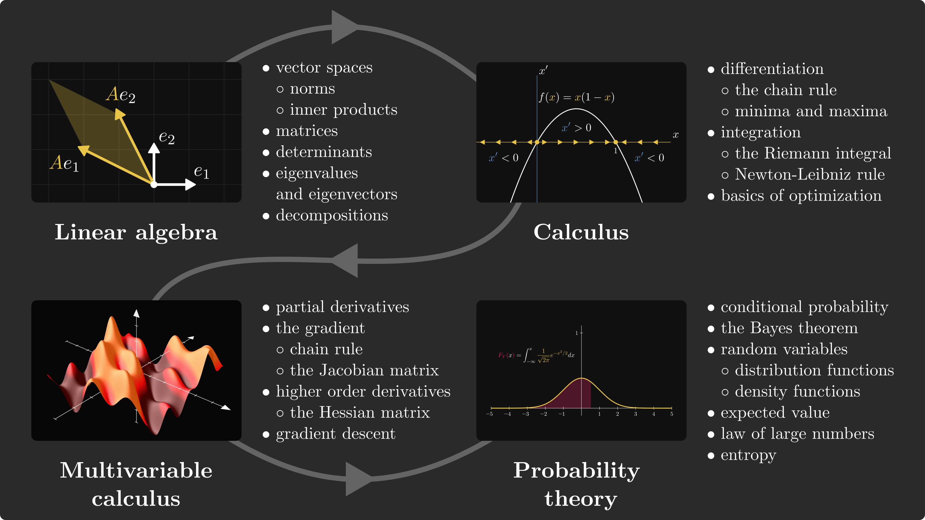
- Vectors and Vector Spaces: Points in space represented by tuples.
- Normed Spaces: Measuring distance (Euclidean, Manhattan, Supremum).
- Matrix Operations: Multiplication as composition of transformations.
- Eigenvalues & SVD: Essential for dimensionality reduction (PCA).
Used to fit models to data through differentiation and integration.
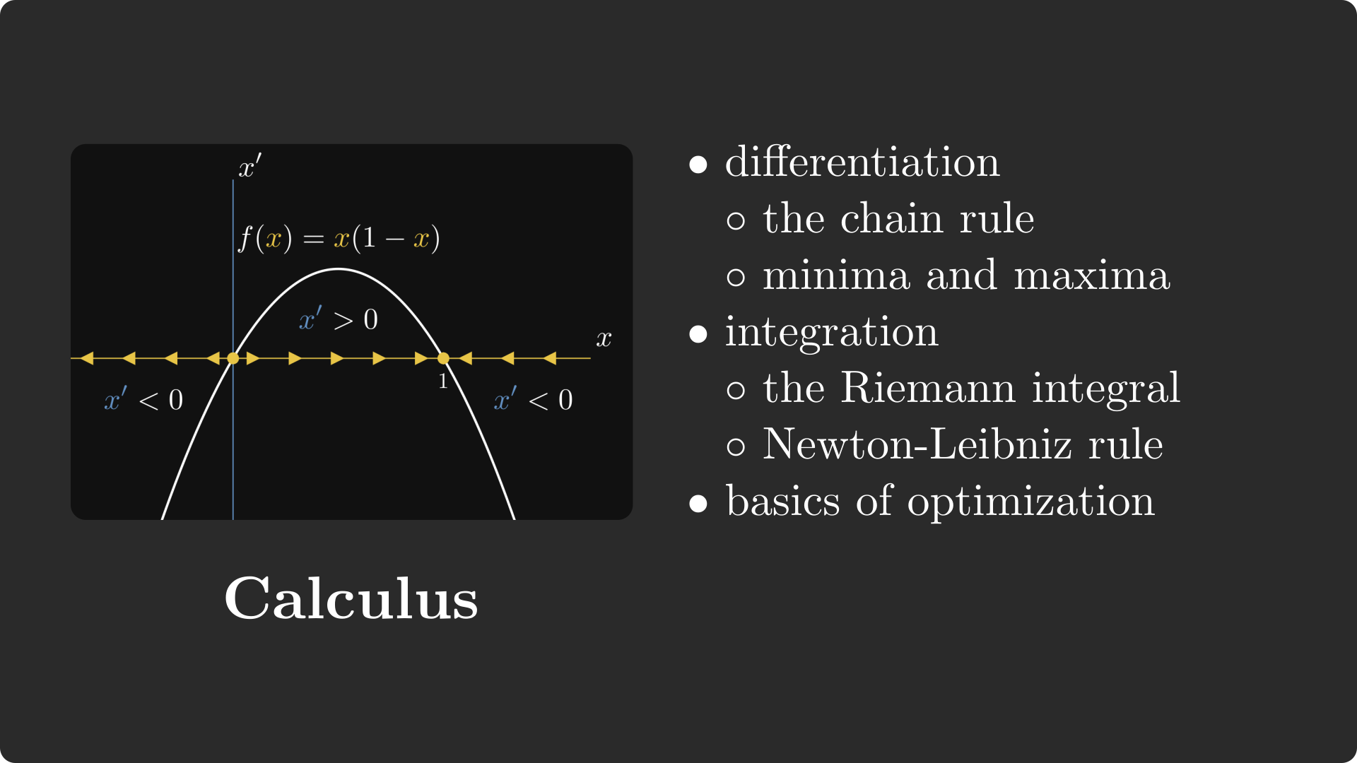
- Derivatives: Tangent slopes for optimization.
- Chain Rule: Core of backpropagation in neural networks.
- Integrals: Area under the curve, used in expected values and entropy.
The foundation of Gradient Descent.
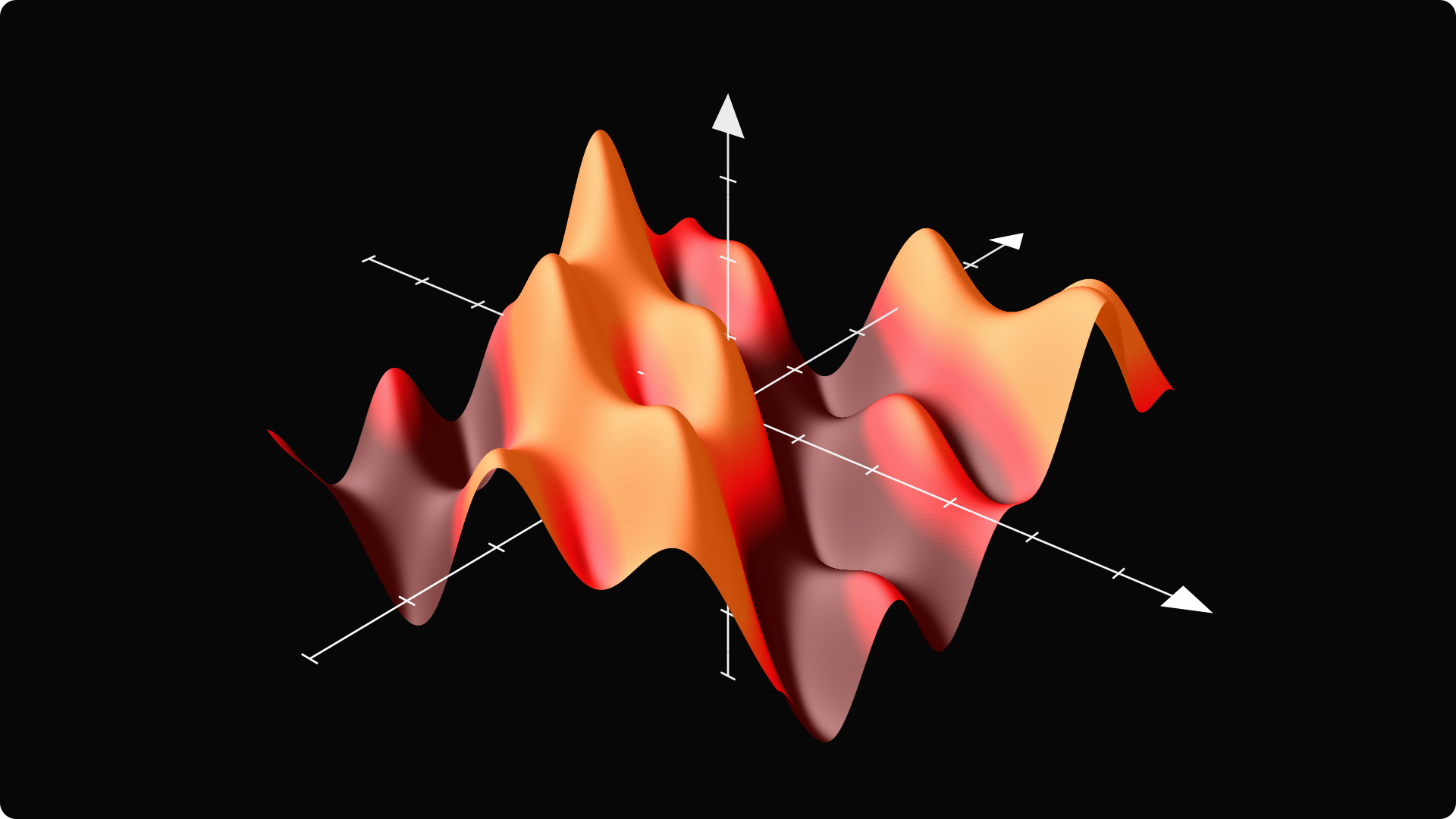
- The Gradient: Vector pointing to the direction of largest increase.
- Hessian Matrix: Higher-order derivatives for determining local minima/maxima.
The mathematical study of chance and uncertainty.
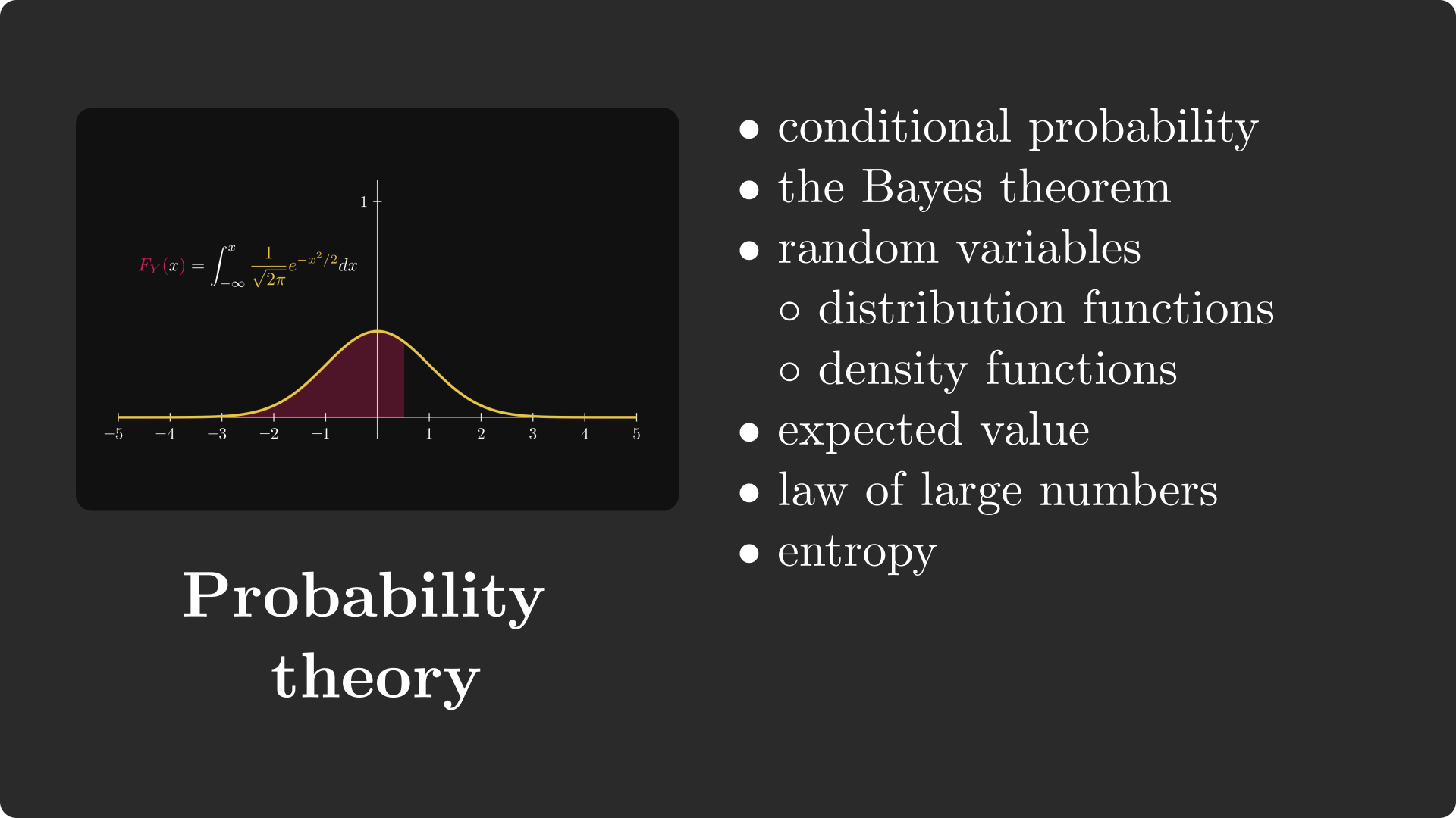
- Bayes' Theorem: Updating priors with new observations.
- Expected Value: Long-run averages, core to loss functions.
- Information Theory: Entropy and Cross-Entropy loss for classification.
For the full detailed roadmap, check out Maths-Roadmap-for-ML-Resources.md