"bpNet: A Bayesian method for estimating network influnece with panel spatial autoregressive model with unobserved factors"

R package for 'A Bayesian Method for Identifying and Explaining Dynamic Network Influence with TSCS Data'.

R source files can be found on the authors' GitHub home page.

Main Reference: Xun Pang and Licheng Liu (2020) "A Bayesian Method for Identifying and Explaining Dynamic Network Influence with TSCS Data".

---

Authors: Xun Pang (Tsinghua); Licheng Liu (MIT)

Date: Sep. 08, 2020

Package: bpNet

Version: 0.0.1 (GitHub version). This package is still under development. Please report bugs!

---

Contents

1. Installation

2. Instructions

3. Example

---

Installation

The development version of the package can be installed from GitHub by typing the following commands:

install.packages('devtools', repos = 'http://cran.us.r-project.org') # if not already installed
devtools::install_github('liulch/bpNet')

The core part of bpNet is written in C++ to accelerate the computing speed, which depends on the packages Rcpp and RcppArmadillo. Pleases install them before running the functions in bpNet.

Notes on installation failures

1. For Rcpp, RcppArmadillo and MacOS "-lgfortran" and "-lquadmath" error, click here for details.
2. Installation failure related to OpenMP on MacOS, click here for a solution.
3. To fix these issues, try installing gfortran 6.1 from here and clang4 R Binaries from here.

---

Instructions

Functional form

We begin with the description of the model to illustrate the syntax of the function bpNet(). The (reduced) functional form of the panel spatial autoregressive (panel SAR) model is: $$ y_{it} = \gamma y_{i,t-1} + \rho_t \sum\limits_{j=1}^{N} w_{ij,t} y_{jt} + X_{it}^{\prime}\beta + Z_{it}^{\prime}\alpha_i + A_{it}^{\prime}\xi_t + \varepsilon_{it} $$ $X_{it}$, $Z_{it}$ and $A_{it}$ are vectors of covariates that have constant, unit-level random and time-level random effects on the outcome respectively. The random effects are assumed to have zero mean. Note that there can be overlapping among $X_{it}$, $Z_{it}$ and $A_{it}$. They may also include exogenous peer effects like $\sum\limits_{j=1}^{N} w_{ij,t} x_{jt,p}$ for some exogenous covariate $\bf{x}_{p}$.

Arguments and options

bpNet() is the main function in the package bpNet. It has several arguments and options for estimating the panel SAR model. We first briefly explain the meaning of each argument and option and then give an illustration using the built-in data of immigration and terrorism. Details about the dataset and the empirical analysis can be found in Bove and Bohmelt (2016). Suppose we have a dataset that contains N units, and each unit is observed repeatedly for T periods.

1. data: a balanced data frame that contains no missing values.
2. W: a $N \times N \times T$ array with each slice a $N \times N$ spatial weight matrix for that period.
3. index: a character vector of length 2 that specifies the variable names of unit and period.
4. Yname: a character value the specifies the outcome variable.
5. Xname: a character vector that specifies the names of covariates that have constant effect.
6. Zname: a character vector that specifies the names of covariates that have unit-level random effect. Default value is `NULL`.
7. Aname: a character vector that specifies the names of covariates that have time-level random effect. Default value is `NULL`.
8. Contextual: a character vector that specifies the names of covariates that have exogenous peer effects. Default value is `NULL`.
9. Contextual.effect: a character value that specifies the effects of the contextual variables. The contextual variables may have constant, unit-level random, time-level random or two-way random effects. Choose from: `"none"`, `"unit"`, `"time"` and `"both"`.
10. lagY: a logical flag that specifies whether to include lagged outcome.
11. force: a character value that specifies whether to include two-way random effects. Choose from: `"none"`, `"unit"`, `"time"` and `"both"`.
12. r: an integer that specifies the number of factors.
13. flasso: a logical flag that specifies whether to perform factor selection.
14. rhoZ: a $T \times p$ matrix of time-varying covariates that explains the spatial autoregressive coefficients.
15. constantRho: a logical flag that specifies whether to set the spatial autoregressive coefficients as constant.
16. randomRho: a logical flag that specifies whether to set the spatial autoregressive coefficients as time-varying.
17. spec: a character value that specifies the state equation of time-varying spatial autoregressive coefficients. Choose from: `"multilevel"`, `"rw"`, and `"ar1`, with `"multilevel"` for a multilevel model, `"rw"` for a random walk process, and `"ar1"` for a stationary AR(1) process.
18. niter: an integer that specifies the number of iterations of the MCMC algorithm.
19. burn: an integer that specifies the number of iterations that are to be burnt-in.

Output

The output of bpNet() is a list of simulated posterior distributions of relevant parameters. It contains the following objects:

1. beta: Simulated posterior distributions for coefficients of covariates (also include the intercept and contextual variables) that have constant effects.
2. rhoy: Simulated posterior distribution for the coefficient of lagged outcome.
3. omega: Simulated posterior distributions for weights of each factor.
4. sigma2: Simulated posterior distribution for variance of the error term.
5. Alpha: Simulated posterior distributions for unit-level random effects.
6. Xi: Simulated posterior distributions for time-level random effects.
7. rho0: Simulated posterior distribution for constant SAR coefficient.
8. Rho: Simulated posterior distributions for time-varying SAR coefficients.
9. kappa: Simulated posterior distribution for the AR1 coefficient in the time-varying SAR coefficients state equation.
10. sigma_n2: Simulated posterior distribution for the variance of the error term in the time-varying SAR coefficients state equation.
11. rhoA: Simulated posterior distributions for the coefficients of the time-varying covariates that explain the SAR coefficients.
12. L: Simulated posterior distributions for the factor loadings.
13. Factor: Simulated posterior distributions for the factors.

Example

We use the built-in dataset of immigration and terrorism to illustrate the functionality of bpNet(). Bove and Bohmelt (2016) use this dataset to study the interdependence of terrorism using immigration as network. We first load the dataset.

set.seed(123456789)
library(bpNet) 
data(bpNet)
ls()

Below is the immigration network in 1986.

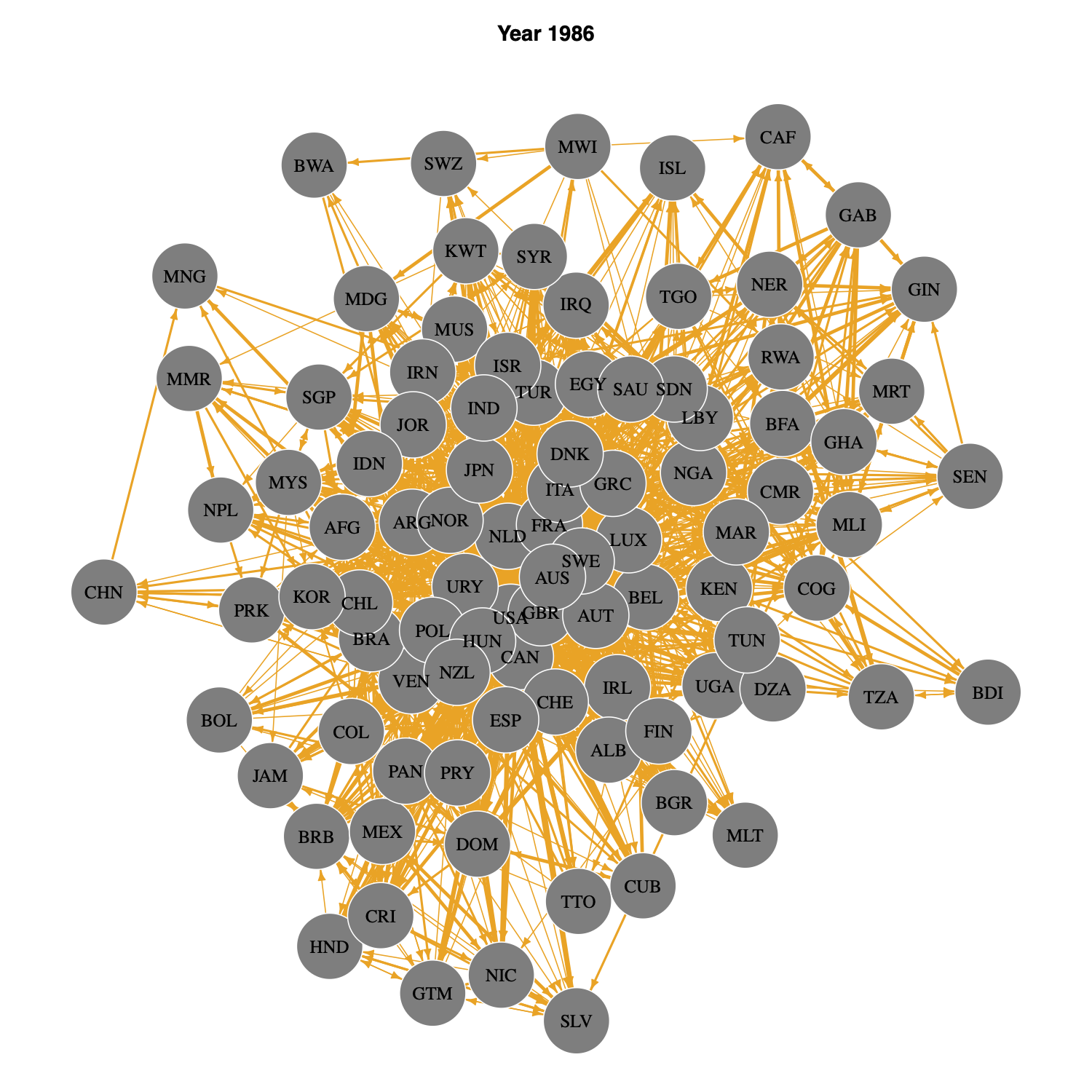
The dataset contains observations for 94 countries spanning 31 years, from 1970 to 2000. Here data is a data frame that contains relevant variables, W is the array of spatial weight matrix, and rhoZ is a numeric vector that measuring network density for each year, which is used to explain the time-varying SAR coefficients. Before estimating the model, we add an intercept term to rhoZ and convert it into a matrix. For a random walk process with local trend, the intercept term is slightly different, i.e. the first period is 1 and all other periods are 0. The intercept vector with each entry equal 1 corresponds to a random walk process with drift term. The total numbers of iteration is set as 35000 and the first 5000 iterations are burn-in. For factor selection, we assume a priori that there are 5 factors and then do factor selection.

mcmc <- 35000
burnin <- 5000

TT <- length(rhoZ)

rhoZ0 <- cbind(c(1, rep(0, TT - 1)), rhoZ)
rhoZ1 <- cbind(1, rhoZ) 

In this demo, we estimate the panel SAR model with time-varying SAR coefficients that either follows a random walk process with local trend or an AR1 process. We type the following code to estimate the model with the two specifications.

## random walk
out1.1 <- bpNet(data = data,   ## a data frame
                W = W,         ## an array N * N * TT, 
                index = c("Uid", "Tid"), ## id and time
                Yname = "Y",
                Xname = c("geddes1", "geddes2","geddes3","geddes4","geddes5", 
                          "logGNI", "logpop", "logarea", "GINI", "Durable", 
                          "AggSF", "ColdWar", "ucdp_type2" ,"ucdp_type3", 
                          "log_iMigrantsBA", "LDV1"),
                Zname = NULL,  
                Aname = NULL,   
                Contextual = c("ucdp_type3"),  
                Contextual.effect = "both",  
                lagY = FALSE,                
                force = "both",             
                r = 5,
                flasso = 1,            
                rhoZ = rhoZ0,  
                constantRho = 0,
                randomRho = 1,     
                spec = "rw",                
                niter = mcmc,
                burn = burnin)

##AR1
out1.2 <- bpNet(data = data,   ## a data frame
                W = W,         ## an array N * N * TT, 
                index = c("Uid", "Tid"), ## id and time
                Yname = "Y",
                Xname = c("geddes1", "geddes2","geddes3","geddes4","geddes5", 
                         "logGNI", "logpop", "logarea", "GINI", "Durable", 
                         "AggSF", "ColdWar", "ucdp_type2" ,"ucdp_type3", 
                         "log_iMigrantsBA", "LDV1"),
                Zname = NULL,  
                Aname = NULL,   
                Contextual = c("ucdp_type3"),  
                Contextual.effect = "both",  
                lagY = FALSE,                
                force = "both",             
                r = 5,
                flasso = 1,            
                rhoZ = rhoZ1,  
                constantRho = 0,
                randomRho = 1,     
                spec = "ar1",                
                niter = mcmc,
                burn = burnin)

We plot the estimated posterior distribution of the error variance under the random walk process specification of SAR coefficients.

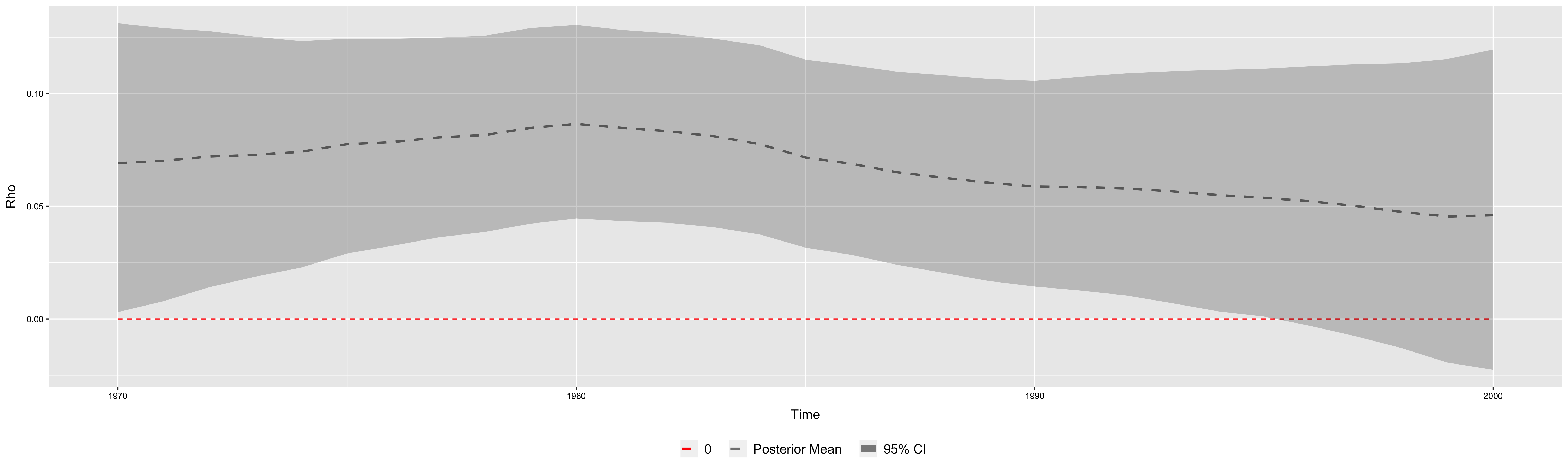
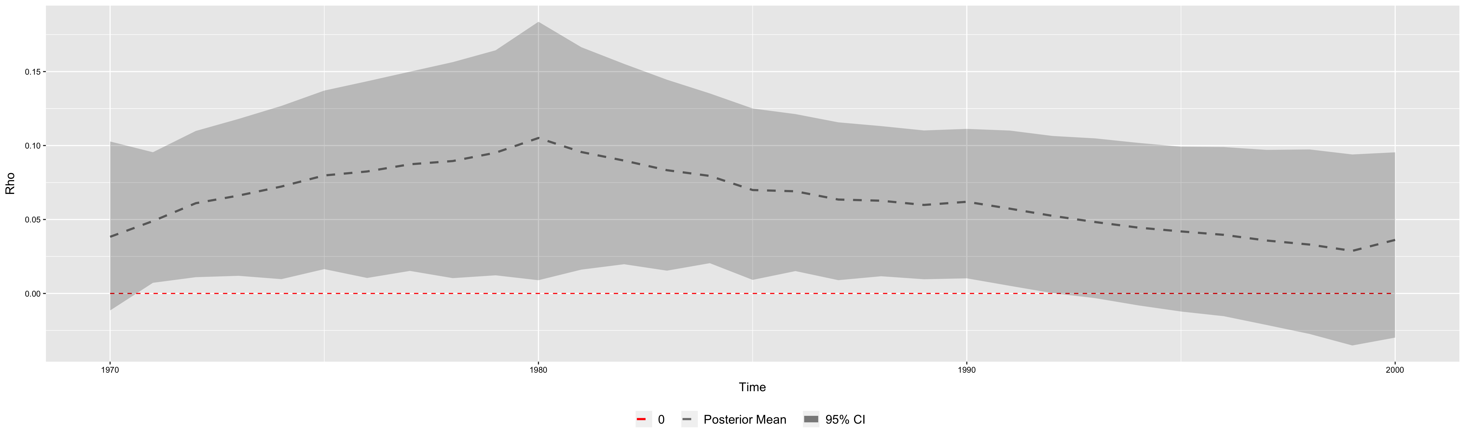
The estimated posterior distribution of SAR coefficients under random walk process and AR1 process specifications are displayed as follows.

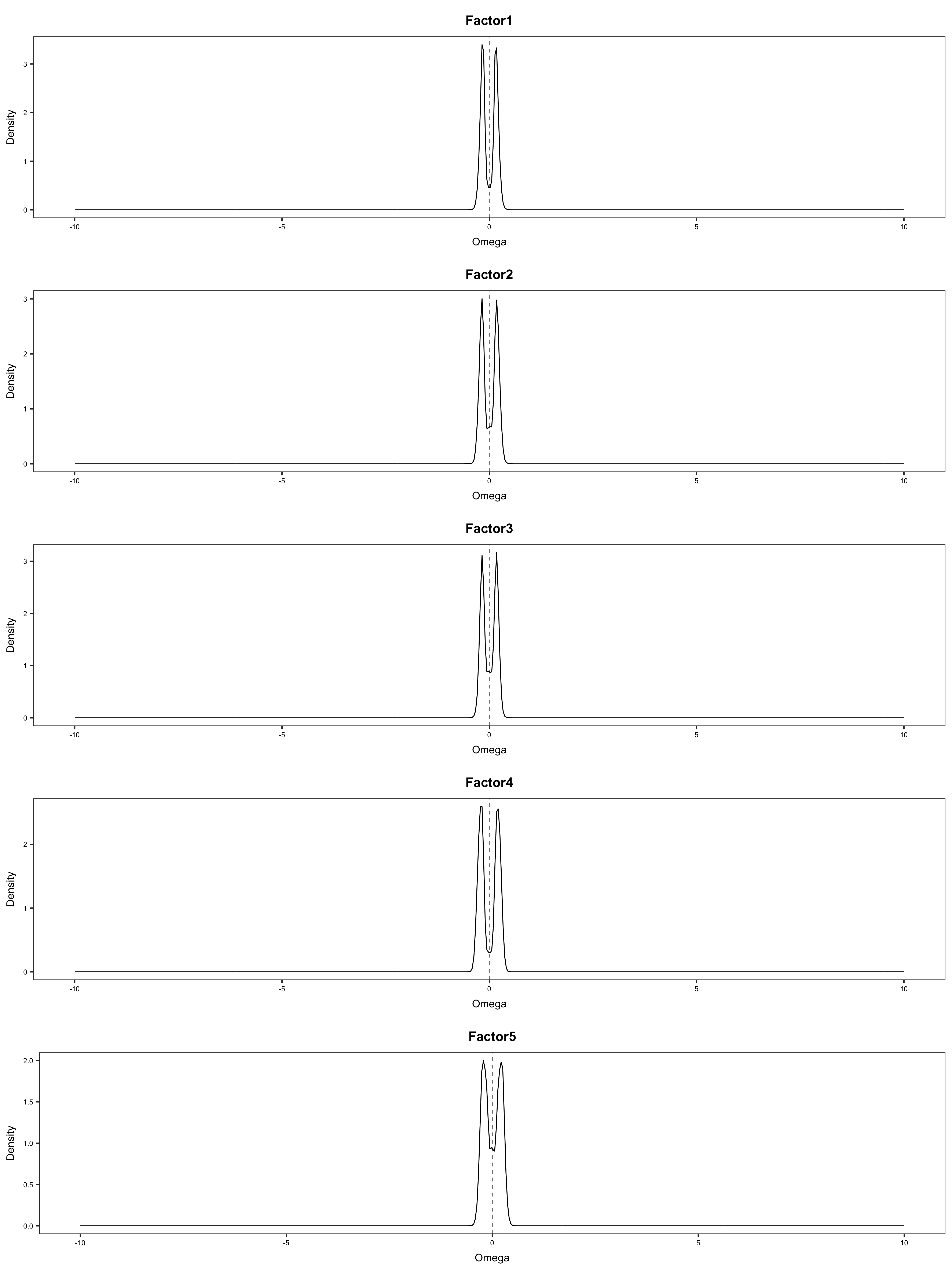
We also show the results of factor selection under the random walk process specification. The bimodal posterior distributions imply that we should include all the 5 factors into the model.

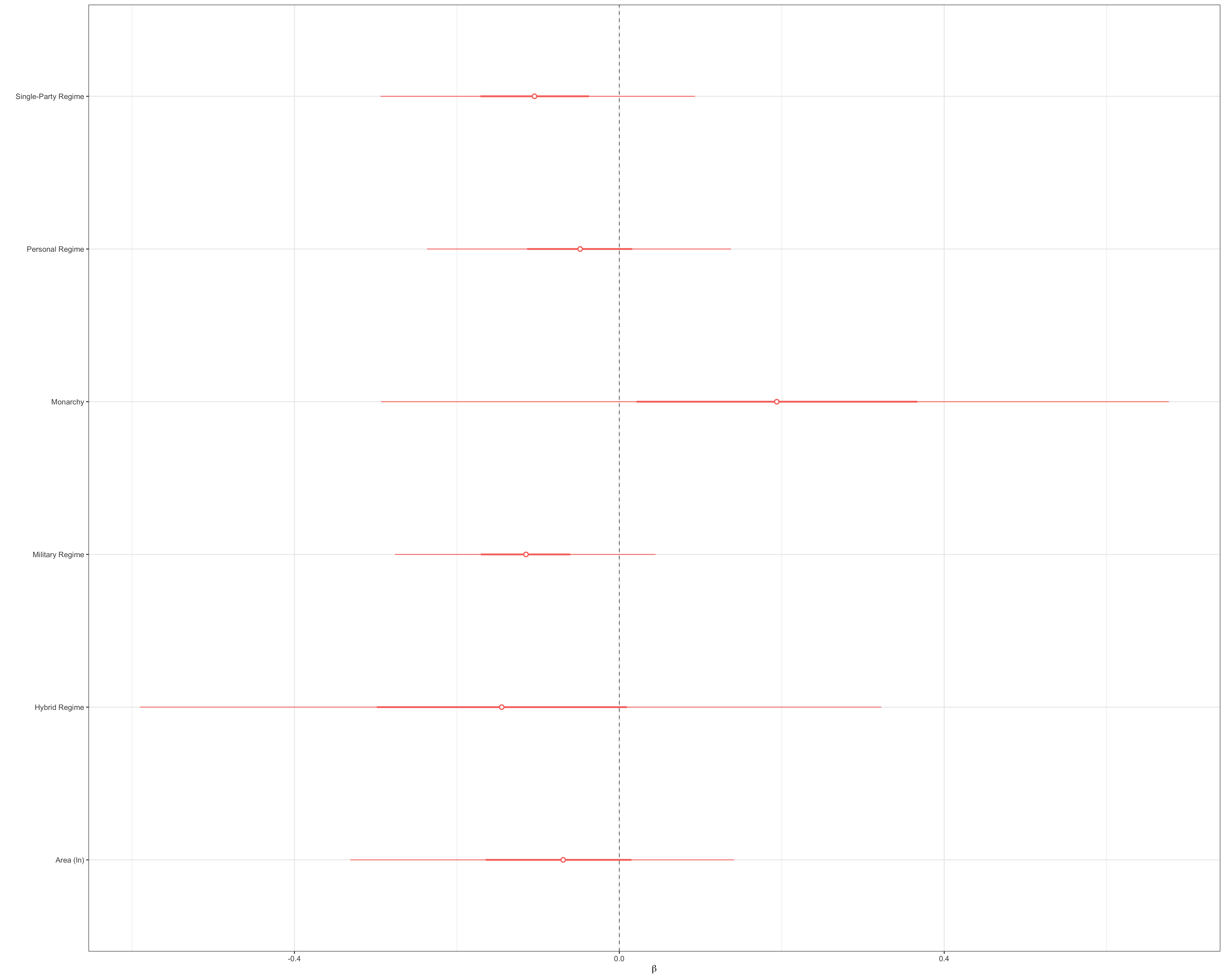
Finally, we report coefficients for a fraction of covariates under the random walk process specification.

\pagebreak

---

---

Addtional References:

Bove, V., & Böhmelt, T. (2016). Does immigration induce terrorism?. The Journal of Politics, 78(2), 572-588.

$\square$