![]()


███╗   ███╗  ██████╗ ██████╗
████╗ ████║ ██╔════╝ ██╔══██╗ ██████╗ ██╗    ██╗███████╗██████╗
██╔████╔██║ ██║      ██║  ██║██╔═══██╗██║    ██║██╔════╝██╔══██╗
██║╚██╔╝██║ ██║      ██████╔╝██║   ██║██║ █╗ ██║█████╗  ██████╔╝
██║ ╚═╝ ██║ ██║      ██╔═══╝ ██║   ██║██║███╗██║██╔══╝  ██╔══██╗
██║     ██║ ╚██████╗ ██║     ╚██████╔╝╚███╔███╔╝███████╗██║  ██║
╚═╝     ╚═╝  ╚═════╝ ╚═╝      ╚═════╝  ╚══╝╚══╝ ╚══════╝╚═╝  ╚═╝
Simple Monte Carlo power analysis for complex models. Find the sample size you need or check if your study has enough power - even with complex models that traditional power analysis can't handle.
It's a Python package, but prefer a graphical interface? MCPower GUI is a standalone desktop app with built-in documentation — no Python installation required. Download ready-to-run executables for Windows, Linux, and macOS from the releases page.
| Model setup | Results |
|---|---|
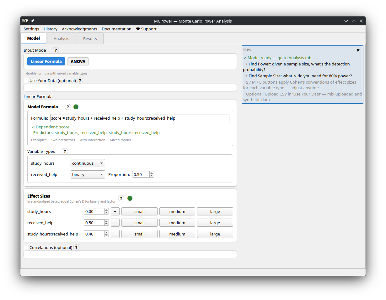 |
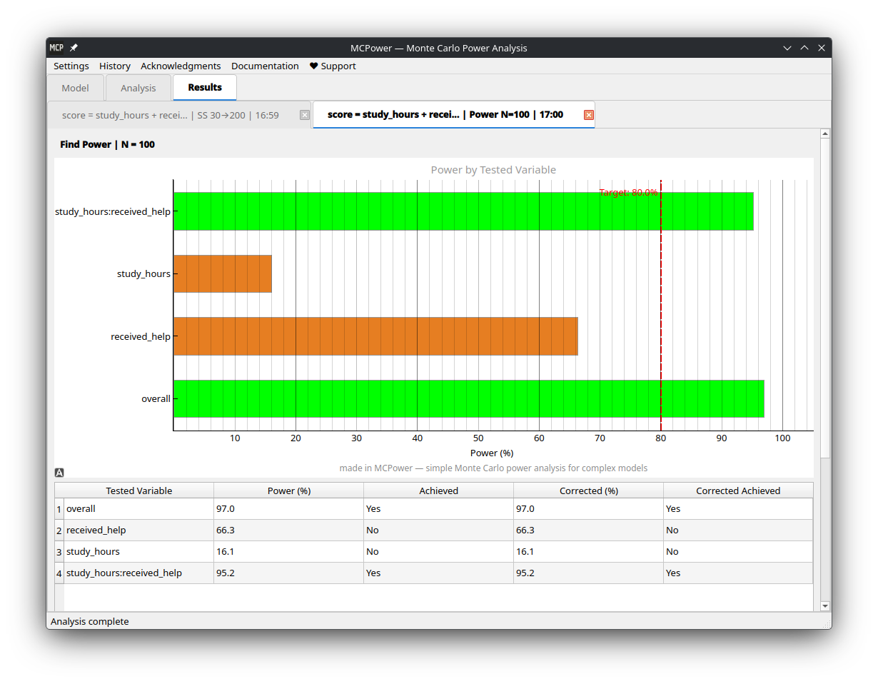 |
Traditional power formulas break down with interactions, correlated predictors, categorical variables, or non-normal data. MCPower simulates instead — generates thousands of datasets like yours, fits your model, and counts how often the effects are detected.
-
Write your formula. Define your model the way you'd write it in R —
outcome = treatment + covariate + treatment*covariate. MCPower parses it, sets up the simulation, and handles dummy coding, interactions, and factor variables automatically. You focus on the research question, not the mechanics. -
Test your assumptions. Real studies rarely match textbook conditions — effect sizes may be smaller than expected, distributions may be skewed, variance may not be constant. Add
scenarios=Trueand MCPower runs your analysis under optimistic, realistic, and worst-case conditions, giving you a range instead of a single number you can't trust. -
All hypotheses at once. MCPower evaluates power for every effect in your model by default. Narrow it down with
target_test="effect1, effect2"when needed. Built-in corrections (Bonferroni, FDR, Holm, Tukey) keep false positive rates under control across multiple comparisons. -
Use your own data. Upload a CSV and MCPower auto-detects variable types (continuous, binary, categorical), preserves real distributions, and handles correlations between predictors. Especially useful when you have pilot data and want your power analysis to reflect actual conditions rather than idealized ones.
-
Mixed models. Clustered and longitudinal data are supported via standard R random-effects syntax —
(1|group)for random intercepts,(1 + x|group)for random slopes, and nested structures like(1|school/classroom).
pip install mcpowerpip install --upgrade mcpower# 0. Import installed package
from mcpower import MCPower
# 1. Define your model (just like R)
model = MCPower("satisfaction = treatment + motivation")
# 2. Set effect sizes (how big you expect effects to be)
model.set_effects("treatment=0.5, motivation=0.3")
# 3. Change the treatment to "binary" (people receive treatment or not).
model.set_variable_type("treatment=binary")
# 4. Find the sample size you need
model.find_sample_size(target_test="treatment", from_size=50, to_size=200, summary="long")Output: "You need N=75 for 80% power to detect the treatment effect"
That's it! 🎉
Real studies rarely match perfect assumptions. MCPower's scenario analysis tests how robust your power calculations are under realistic conditions.
# Test robustness with scenario analysis
model.find_sample_size(
    target_test="treatment",
    from_size=50, to_size=300,
    scenarios=True  # 🔥 The magic happens here
)
Output:
SCENARIO SUMMARY
================================================================================

Uncorrected Sample Sizes:
Test                                     Optimistic   Realistic    Doomer
-------------------------------------------------------------------------------
treatment                                75           85           100
================================================================================
What each scenario means:
- Optimistic: Your ideal conditions (original settings)
- Realistic: Moderate real-world complications (small effect variations, mild assumption violations)
- Doomer: Conservative estimate (larger effect variations, stronger assumption violations)
💡 Pro tip: Use the Realistic scenario for planning. If Doomer is acceptable, you're really safe!
Effect sizes tell you how much the outcome changes when predictors change.
- Effect size = 0.5 means the outcome increases by 0.5 standard deviations when:
- Continuous variables: Predictor increases by 1 standard deviation
- Binary variables: Predictor changes from 0 to 1 (e.g., control → treatment)
- Factor variables: Each level compared to reference level (first level)
Practical examples:
model.set_effects("treatment=0.5, age=0.3, income=0.2")treatment=0.5: Treatment increases outcome by 0.5 SD (medium-large effect)age=0.3: Each 1 SD increase in age → 0.3 SD increase in outcomeincome=0.2: Each 1 SD increase in income → 0.2 SD increase in outcome
Effect size guidelines:
- 0.1 = Small effect (detectable but modest)
- 0.25 = Medium effect (clearly noticeable)
- 0.4 = Large effect (substantial impact)
Effect size guidelines (binary variables):
- 0.2 = Small effect (detectable but modest)
- 0.5 = Medium effect (clearly noticeable)
- 0.8 = Large effect (substantial impact)
Your uploaded data is automatically standardized (mean=0, SD=1) so effect sizes work the same way whether you use synthetic or real data.
from mcpower import MCPower

# RCT with treatment + control variables
model = MCPower("outcome = treatment + age + baseline_score")
model.set_effects("treatment=0.6, age=0.2, baseline_score=0.8")
model.set_variable_type("treatment=binary")  # 0/1 treatment

# Find sample size for treatment effect with scenario analysis
model.find_sample_size(target_test="treatment", from_size=100, to_size=500,
by=50, scenarios=True)from mcpower import MCPower
# Test if treatment effect depends on user type
model = MCPower("conversion = treatment + user_type + treatment*user_type")
model.set_effects("treatment=0.4, user_type=0.3, treatment:user_type=0.5")
model.set_variable_type("treatment=binary, user_type=binary")
# Check power robustness for the interaction
model.find_power(sample_size=400, target_test="treatment:user_type", scenarios=True)from mcpower import MCPower
# Study with 3 treatment groups and 4 education levels
model = MCPower("wellbeing = treatment + education + age")
model.set_variable_type("treatment=(factor,3), education=(factor,4)")
# Set effects for each factor level (vs. reference level 1)
model.set_effects("treatment[2]=0.4, treatment[3]=0.6, education[2]=0.3, education[3]=0.5, education[4]=0.7, age=0.2")
# Find sample size for treatment effects
model.find_sample_size(target_test="treatment[2], treatment[3]", scenarios=True)from mcpower import MCPower
# Predictors are often correlated in real data
model = MCPower("wellbeing = income + education + social_support")
model.set_effects("income=0.4, education=0.3, social_support=0.6")
model.set_correlations("corr(income, education)=0.5, corr(income, social_support)=0.3")
# Find sample size for any effect
model.find_sample_size(target_test="all", from_size=200, to_size=800,
by=100, scenarios=True)# Binary, factors, skewed, or other distributions
model.set_variable_type("treatment=binary, condition=(factor,3), income=right_skewed, age=normal")
# Binary with custom proportions (30% get treatment)
model.set_variable_type("treatment=(binary,0.3)")
# Factors with custom group sizes (20%, 50%, 30%)
model.set_variable_type("condition=(factor,0.2,0.5,0.3)")# Factors automatically create dummy variables
model = MCPower("outcome = treatment + education")
model.set_variable_type("treatment=(factor,3), education=(factor,4)")
# Set effects for specific levels (level 1 is always reference)
model.set_effects("treatment[2]=0.5, treatment[3]=0.7, education[2]=0.3, education[3]=0.4, education[4]=0.6")Use upload_data() to preserve real-world distribution shapes and relationships:
import csv

# Load your data (no extra dependencies needed)
with open("my_data.csv") as f:
    reader = csv.DictReader(f)
    rows = list(reader)
data = {col: [float(r[col]) for r in rows] for col in ["hp", "wt", "cyl"]}

# Upload with automatic type detection
model = MCPower("mpg = hp + wt + cyl")
model.upload_data(data)
model.set_effects("hp=0.5, wt=0.3, cyl[6]=0.2, cyl[8]=0.4")
model.find_power(sample_size=100)
Or with pandas (optional: pip install pandas):
import pandas as pd
data = pd.read_csv("my_data.csv")
model.upload_data(data[["hp", "wt", "cyl"]])
Auto-Detection
Variables are automatically classified based on unique values:
- 1 unique value: Dropped (constant)
- 2 unique values: Binary variable
- 3-6 unique values: Factor/categorical variable
- 7+ unique values: Continuous variable
Correlation Preservation Modes
Control how correlations are handled with the preserve_correlation parameter:
# No correlation preservation
model.upload_data(data, preserve_correlation="no")

# Partial: Compute correlations from data, merge with user settings
model.upload_data(data, preserve_correlation="partial")

# Strict: Bootstrap whole rows to preserve exact relationships (default)
model.upload_data(data, preserve_correlation="strict")
Override Auto-Detection
Force specific variable types:
model.upload_data(
    data,
    data_types={"cyl": "factor", "hp": "continuous"}
)# Testing multiple effects? Control false positives
model.find_power(
sample_size=200,
target_test="treatment,covariate,treatment:covariate",
correction="Benjamini-Hochberg",
scenarios=True # Test robustness too!
)# Compare specific factor levels with Tukey correction
model = MCPower("outcome = group + covariate")
model.set_variable_type("group=(factor,3)")
model.set_effects("group[2]=0.4, group[3]=0.6, covariate=0.3")
# Use "vs" syntax for pairwise comparisons + correction="tukey"
model.find_power(
sample_size=150,
target_test="group[1] vs group[2], group[1] vs group[3]",
correction="tukey"
)# Add specific violations via custom scenario configs
model.set_scenario_configs({
"my_test": {"heterogeneity": 0.2, "heteroskedasticity": 0.15}
})
# Run with scenario variations
model.find_sample_size(target_test="treatment", scenarios=True)from mcpower import MCPower
# Random intercept — clustered data
model = MCPower("satisfaction ~ treatment + motivation + (1|school)")
model.set_cluster("school", ICC=0.2, n_clusters=20)
model.set_effects("treatment=0.5, motivation=0.3")
model.set_variable_type("treatment=binary")
model.set_max_failed_simulations(0.10)
model.find_power(sample_size=1000) # 1000/20 = 50 per cluster
# Random slopes — effect varies across clusters
model = MCPower("y ~ x1 + (1 + x1|school)")
model.set_cluster("school", ICC=0.2, n_clusters=20,
random_slopes=["x1"], slope_variance=0.1,
slope_intercept_corr=0.3)
model.set_effects("x1=0.5")
model.set_max_failed_simulations(0.30)
model.find_power(sample_size=1000)
# Nested random effects — students in classrooms in schools
model = MCPower("y ~ treatment + (1|school/classroom)")
model.set_cluster("school", ICC=0.15, n_clusters=10)
model.set_cluster("classroom", ICC=0.10, n_per_parent=3) # 3 classrooms per school
model.set_effects("treatment=0.5")
model.set_max_failed_simulations(0.30)
model.find_power(sample_size=1500)See the Mixed-Effects Models documentation for detailed documentation on all model types, parameters, and design recommendations.
MCPower's mixed-effects solver is validated against R's lme4 across 95 scenarios using four independent strategies — all 230 scenario-strategy combinations pass.
# To make a more precise estimation, consider increasing the number of simulations.
model.set_simulations(10000)

# Parallelization is enabled by default for mixed models ("mixedmodels" mode).
# To enable it for all analyses:
model.set_parallel(True)

# To disable parallelization entirely:
model.set_parallel(False)# Set a seed for reproducible results
model.set_seed(42)
# All set_* methods support chaining
model.set_effects("x1=0.5").set_variable_type("x1=binary").set_alpha(0.01)
# Get results as a Python dict for further processing
results = model.find_power(sample_size=200, return_results=True)
# Custom progress callback (useful in notebooks or GUIs)
model.find_power(sample_size=200, progress_callback=lambda cur, tot: print(f"{cur}/{tot}"))
# Disable progress output entirely
model.find_power(sample_size=200, progress_callback=False)| Want to... | Use this |
|---|---|
| Find required sample size | model.find_sample_size(target_test="effect_name") |
| Check power for specific N | model.find_power(sample_size=150, target_test="effect_name") |
| Test robustness | Add scenarios=True to either method |
| Detailed output with plots | Add summary="long" to either method |
| Test overall model | target_test="overall" |
| Test multiple effects | target_test="effect1, effect2" or "all" |
| Binary variables | model.set_variable_type("var=binary") |
| Factor variables | model.set_variable_type("var=(factor,3)") |
| Factor effects | model.set_effects("var[2]=0.5, var[3]=0.7") |
| Correlated predictors | model.set_correlations("corr(var1, var2)=0.4") |
| Multiple testing correction | Add correction="FDR", "Holm", "Bonferroni", or "Tukey" |
| Post-hoc pairwise comparison | target_test="group[1] vs group[2]" with correction="tukey" |
| Mixed model (random intercept) | MCPower("y ~ x + (1|group)") + model.set_cluster(...) |
| Random slopes | MCPower("y ~ x + (1+x|group)") + set_cluster(..., random_slopes=["x"], slope_variance=0.1) |
| Nested random effects | MCPower("y ~ x + (1|A/B)") + two set_cluster() calls |
| Reproducible results | model.set_seed(42) |
| Get results as dict | Add return_results=True to either method |
| Stricter significance | model.set_alpha(0.01) |
| Target 90% power | model.set_power(90) |
✅ Use MCPower when you have:
- Interaction terms (
treatment*covariate) - Categorical variables with multiple levels
- Binary or non-normal variables
- Correlated predictors
- Multiple effects to test
- Need to test assumption robustness
- Complex models where traditional power analysis fails
✅ Use Scenario Analysis when:
- Planning important studies
- Working with messy real-world data
- Effect sizes are uncertain
- Want conservative sample size estimates
- You need confidence in your numbers
❌ Use traditional power analysis for:
- For models that are not yet implemented
- For simple models where all assumptions are clearly met.
- For large analyses with tens of thousands of observations, tiny effects, or very low alpha levels.
Traditional power analysis assumes perfect conditions. MCPower's scenarios add realistic "messiness":
| Scenario | What's Different | When to Use |
|---|---|---|
| Optimistic | Your exact settings | Best-case planning |
| Realistic | Mild effect variations, small assumption violations | Recommended for most studies |
| Doomer | Larger effect variations, stronger assumption violations | Conservative/worst-case planning |
Behind the scenes, scenarios randomly vary:
- Effect sizes between participants
- Correlation strengths
- Variable distributions
- Assumption violations
This gives you a range of realistic outcomes instead of a single optimistic estimate.
📚 Advanced Features (Click to expand)
model.set_variable_type("""
    treatment=binary,           # 0/1 with 50% split
    ses=(binary,0.3),          # 0/1 with 30% split
    condition=(factor,3),       # 3-level factor (equal proportions)
    education=(factor,0.2,0.5,0.3), # 3-level factor (custom proportions)
    age=normal,                # Standard normal (default)
    income=right_skewed,       # Positively skewed
    depression=left_skewed,    # Negatively skewed
    response_time=high_kurtosis, # Heavy-tailed
    rating=uniform             # Uniform distribution
""")# Factor variables are categorical with multiple levels
model = MCPower("outcome = treatment + education")
# Create factors
model.set_variable_type("treatment=(factor,3), education=(factor,4)")
# This creates dummy variables automatically:
# treatment[2], treatment[3] (treatment[1] is reference)
# education[2], education[3], education[4] (education[1] is reference)
# Set effects for specific levels
model.set_effects("treatment[2]=0.5, treatment[3]=0.7, education[2]=0.3")
# Each non-reference level needs its own effect
model.set_effects("treatment[2]=0.5, treatment[3]=0.7")
# Important: Factors cannot be used in correlations
# This will error: model.set_correlations("corr(treatment, education)=0.3")
# Use continuous variables only: model.set_correlations("corr(age, income)=0.3")import numpy as np
# Full correlation matrix for 3 CONTINUOUS variables only
# (Factors are excluded from correlation matrices)
corr_matrix = np.array([
[1.0, 0.4, 0.6], # Variable 1 with others
[0.4, 1.0, 0.2], # Variable 2 with others
[0.6, 0.2, 1.0] # Variable 3 with others
])
model.set_correlations(corr_matrix)# Adjust for your needs
model.set_power(90) # Target 90% power instead of 80%
model.set_alpha(0.01) # Stricter significance (p < 0.01)
model.set_simulations(10000) # High precision (slower)Use test_formula to generate data with one model but test with a simpler one -- useful for evaluating the power impact of omitting variables:
# Generate with 3 predictors, test with 2 (omitting x3)
model = MCPower("y = x1 + x2 + x3")
model.set_effects("x1=0.5, x2=0.3, x3=0.2")
model.find_power(100, test_formula="y = x1 + x2")

# Generate with clusters, test without (ignoring clustering)
model = MCPower("y ~ treatment + (1|school)")
model.set_cluster("school", ICC=0.2, n_clusters=20)
model.set_effects("treatment=0.5")
model.find_power(1000, test_formula="y ~ treatment")
See the Test Formula Tutorial for details.
# These are equivalent:
"y = x1 + x2 + x1:x2"        # Assignment style
"y ~ x1 + x2 + x1:x2"        # R-style formula
"x1 + x2 + x1:x2"            # Predictors only

# Interactions:
"x1*x2"         # Main effects + interaction (x1 + x2 + x1:x2)
"x1:x2"         # Interaction only
"x1*x2*x3" # All main effects + all interactions# String format (recommended)
model.set_correlations("corr(x1, x2)=0.3, corr(x1, x3)=-0.2")
# Shorthand format
model.set_correlations("(x1, x2)=0.3, (x1, x3)=-0.2")
# Note: Factor variables cannot be correlated
# Only use continuous/binary variables in correlations- Python ≥ 3.10
- NumPy (≥1.26.0), matplotlib, joblib, tqdm
- pandas (optional, for DataFrame input — install with
pip install mcpower[pandas])
Full documentation is available at freestylerscientist.pl/mcpower, including:
- Quick Start
- Model Specification
- Variable Types
- Effect Sizes
- Mixed-Effects Models (random intercepts, slopes, nested effects)
- ANOVA & Post-Hoc Tests
- Scenario Analysis
- API Reference
- Issues: GitHub Issues
- Questions: pawellenartowicz@europe.com
- ✅ Linear Regression
- ✅ Scenarios, robustness analysis
- ✅ Factor variables (categorical predictors)
- ✅ C++ native backend (pybind11 + Eigen, 3x speedup)
- ✅ Mixed Effects Models (random intercepts, random slopes, nested effects) — validated against lme4
- 🚧 Logistic Regression (coming soon)
- ✅ ANOVA (factor variables as ANOVA, post-hoc pairwise comparisons)
- ✅ Guide about methods, corrections
- 📋 2 groups comparison with alternative tests
- 📋 Robust regression methods
GPL v3. If you use MCPower in research, please cite:
Lenartowicz, P. (2025). MCPower: Monte Carlo Power Analysis for Complex Statistical Models (Version ) [Computer software]. Zenodo. https://doi.org/10.5281/zenodo.16502734
Replace <your version> with the version you used — check with import mcpower; print(mcpower.__version__).
@software{mcpower2025,
  author    = {Lenartowicz, Pawe{\l}},
  title     = {{MCPower}: Monte Carlo Power Analysis for Complex Statistical Models},
  year      = {2025},
  publisher = {Zenodo},
  doi       = {10.5281/zenodo.16502734},
  url       = {https://doi.org/10.5281/zenodo.16502734}
}
🚀 Ready to start? Copy one of the examples above and adapt it to your study!
I created this project for free without receiving any payment, and if you'd like to support my work, donations are appreciated!