A Tutorial and Usage

if(!require("devtools")) install.packages("devtools")
library(devtools)
install_github("xielab2017/EasyMicroPlot",subdir='Version_0.5.0')
# When something is wrong, please try this below
install_github("xielab2017/EasyMicroPlot",subdir='Version_0.5.0',upgrade = 'never')
## Analysis and results are generated in the output folder

 EMP_MICRO(EMP$micro,EMP$mapping)

## The mapping and microbial relative abundance files have already been deposited in the working directory.
## Users only have to activate easy mode to perform a complete workflow with default parameters and generate results in the working-space.
## Demo data at this repository: Tutorial data/Easy_mode_data.7z

 EMP_MICRO()
.Result/
├── RFCV_result
│   ├── Imprortance
│   ├── model
│   └── taxonomy
├── alpha_result
│   ├── Post-Hoc
│   ├── data
│   ├── html
│   └── pic
├── beta_result
│   ├── bray_0.001_0.7
│   └── jaccard_0.001_0.7
├── cooc_result
│   └── pic
├── core_data
│   ├── species_0.001_70%.txt
│   └── species_0.001_70%_info.txt
└── structure_result
    ├── pic
    ├── taxonomy
    └── top_abundance
## Data preparation
 meta_data <- EMP$meta
 meta_data <- na.omit(meta_data)
 meta_data <- meta_data[meta_data$Diarrhea=='n'&meta_data$Astriction=='n'&meta_data$Antibiotics=='n'&meta_data$Synbiotics=='n',]


## Identify the categorical and continuous variables
 col_str <- 'MetS'
 col_num <- colnames(meta_data)[!colnames(meta_data)%in%c('SampleID','MetS','Diarrhea','Astriction','Antibiotics','Synbiotics')]


## For regroup of meta data
re <- EMP_META(data = meta_data,estimate_group = 'MetS',missing_plot = F,new_col_id = 'Group',col_str = col_str,
                   col_num = col_num,keep_col = 'SampleID',regroup = T,clust_min = 2,clust_max = 9)

## For table generation
 re$summary$summary_table

## For detailed summary of meta data
 re$summary$summary_info

## Show cluster details
 re$regroup$regroup_info

## Show regroup results
 new_group <- re$regroup$regroup_data
## Prepare the bacteria taxa data
 core_data <- data_filter(data = EMP$micro,design = EMP$mapping,
                           min_relative = 0.001,min_ratio = 0.7)
 sp <- core_data$filter_data$species


## Analysis and plot
## When ** cor_output = T **, cooc picture is generated in working directory.
 cor_re <- EMP_COR(data = sp,meta=meta,cor_output = T,method = 'spearman')
## Load data
 library(EasyMicroPlot)
 data(EMP)
## For summary of meta data
 meta <- meta_summary(EMP$meta,estimate_group = 'MetS',keep_col = 'SampleID')

## For table
 meta$summary_table

## For a detailed summary of meta data
 meta$summary_info
   Aginomoto        Animal_oil        Plant_oil         Salt           Sauce
 Min.   :  0.00   Min.   :   0.00   Min.   :   0   Min.   :  0.0   Min.   :  0.00
 1st Qu.:  0.00   1st Qu.:   0.00   1st Qu.: 680   1st Qu.: 67.0   1st Qu.:  0.00
 Median :  0.00   Median :   0.00   Median :1000   Median :100.0   Median :  0.00
 Mean   : 18.89   Mean   :  24.92   Mean   :1209   Mean   :115.2   Mean   : 25.42
 3rd Qu.: 25.00   3rd Qu.:   0.00   3rd Qu.:1500   3rd Qu.:133.0   3rd Qu.: 25.00
 Max.   :200.00   Max.   :1250.00   Max.   :5333   Max.   :400.0   Max.   :500.00
 NA's   :17       NA's   :14        NA's   :23     NA's   :28      NA's   :11
   Soy_sauce          Sugar        Fruit_juice         Fruits           Grains
 Min.   :   0.0   Min.   :  0.0   Min.   :     0   Min.   :     0   Min.   :     0
 1st Qu.:  83.0   1st Qu.:  0.0   1st Qu.:     0   1st Qu.: 27124   1st Qu.: 51025
 Median : 150.0   Median : 10.5   Median :     0   Median : 54750   Median : 73000
 Mean   : 217.5   Mean   : 40.8   Mean   :  7030   Mean   : 70810   Mean   : 83152
 3rd Qu.: 250.0   3rd Qu.: 50.0   3rd Qu.:  4350   3rd Qu.: 91250   3rd Qu.:109226
 Max.   :6667.0   Max.   :750.0   Max.   :182500   Max.   :547500   Max.   :376500
 NA's   :21       NA's   :20
    Red_wine        Rice_wine         H_alcohol       L_alcohol         Livestock
 Min.   :     0   Min.   :    0.0   Min.   :    0   Min.   :    0.0   Min.   :     0
 1st Qu.:     0   1st Qu.:    0.0   1st Qu.:    0   1st Qu.:    0.0   1st Qu.: 10950
 Median :     0   Median :    0.0   Median :    0   Median :    0.0   Median : 23860
 Mean   :  2319   Mean   :  288.3   Mean   : 1105   Mean   :  221.9   Mean   : 33627
 3rd Qu.:   900   3rd Qu.:    0.0   3rd Qu.:    0   3rd Qu.:    0.0   3rd Qu.: 42675
 Max.   :234000   Max.   :54750.0   Max.   :54750   Max.   :18250.0   Max.   :182500

   Vegetables          MetS     Diarrhea   Astriction Antibiotics Synbiotics
 Min.   :     0   Cases  :154   n   :573   n   :561   n   :560    n   :531
 1st Qu.: 73000   Control:464   y   : 41   y   : 53   y   : 52    y   : 80
 Median :109500                 NA's:  4   NA's:  4   NA's:  6    NA's:  7
 Mean   :127451
 3rd Qu.:182500
 Max.   :821250
## Load data
 library(EasyMicroPlot)
 data(EMP)

## Data preparation
 meta_data <- EMP$meta
 meta_data <- na.omit(meta_data)
 meta_data <- meta_data[meta_data$Diarrhea=='n'&meta_data$Astriction=='n'&meta_data$Antibiotics=='n'&meta_data$Synbiotics=='n',]


## Identify the categorical and continuous variables
 col_str <- 'MetS'
 col_num <- colnames(meta_data)[!colnames(meta_data)%in%c('SampleID','MetS','Diarrhea','Astriction','Antibiotics','Synbiotics')]


## For regroup of meta data
 re <- meta_regroup(data = meta_data,new_col_id = 'Group',col_str = col_str,
                   col_num = col_num,keep_col = 'SampleID',regroup = T,clust_min = 2,clust_max = 9)
***********************************************************************
*** : The best number of clusters for Continuous variable data is  2

*** : The best number of clusters for Categorical variable data is  2


                   ***** Conclusion *****

***:  According to the majority rule, the best number of clusters is  4


***********************************************************************
## Show cluster details
 re$regroup_info
$data_num_clust_best
[1] "2"

$data_str_clust_best
[1] 2

$data_clust_best
[1] 4

$data_num_clust_plot
## Show regroup result
 new_group <- re$regroup_data
## Load data
 library(EasyMicroPlot)
 data(EMP)

## Result
 core_data <- data_filter(data = EMP$micro,design = EMP$mapping,min_relative = 0.001,min_ratio = 0.7)
## Load data
library(EasyMicroPlot)
data(EMP)
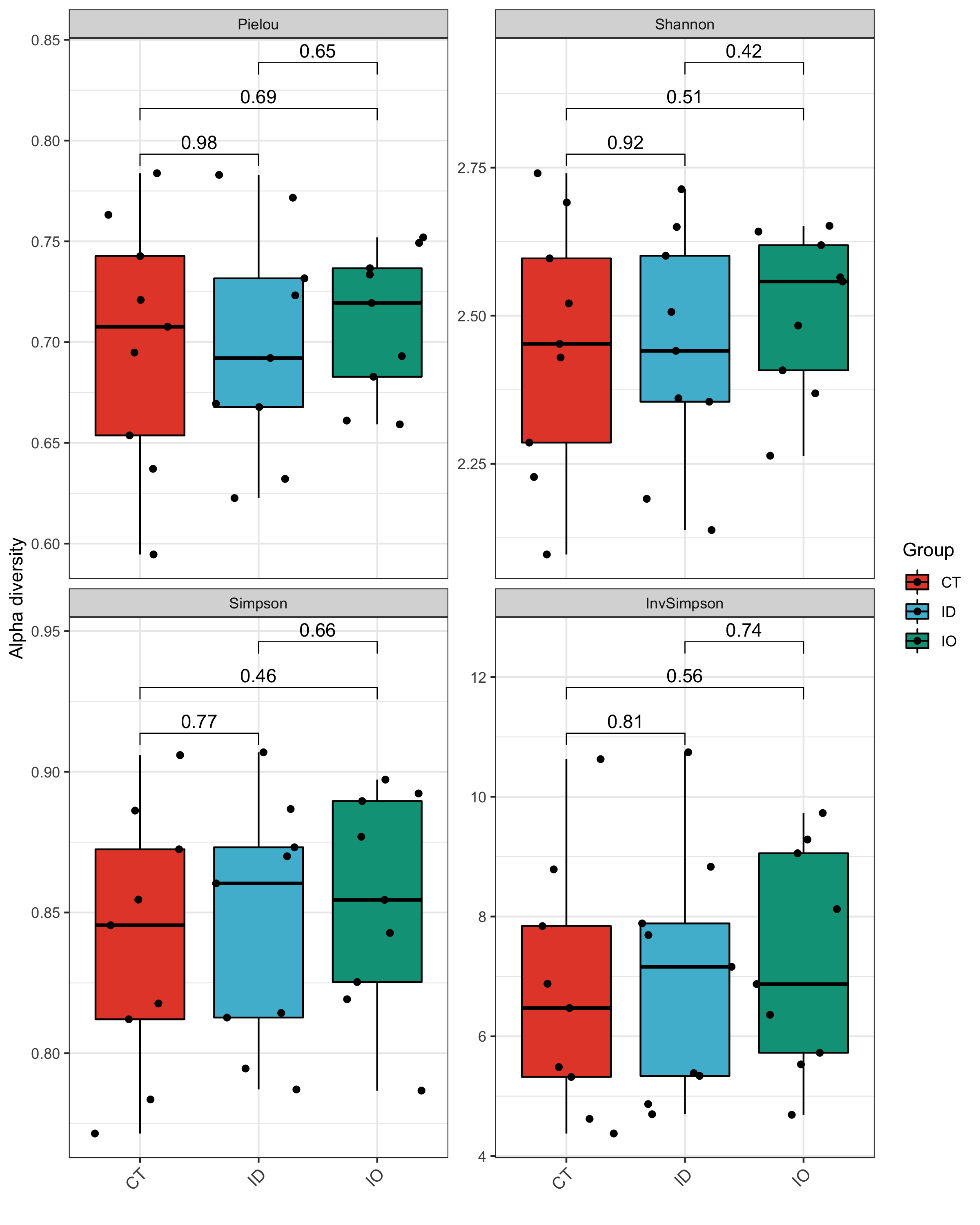
## For Student-Test in comparation
alpha_re <- alpha_plot(data = EMP$micro,design = EMP$mapping,min_relative = 0.001,min_ratio = 0.7,
method = 'ttest')
## For one-way ANOVA and Post Hoc test
alpha_re <- alpha_plot(data = EMP$micro,design = EMP$mapping,min_relative = 0.001,min_ratio = 0.7,
method = 'LSD')
## Support ggplot theme parameters
library(ggplot2)
newtheme=newtheme_slope=theme(axis.text.x =element_text(angle = 90, hjust = -1,size = 15),
axis.title=element_text(size=15,face="bold",colour = 'black'))
alpha_re=alpha_plot(data = EMP$micro,design = EMP$mapping,min_relative = 0.001,min_ratio = 0.7,
method = 'ttest',mytheme = newtheme)
## Plot
alpha_re$plot$species$pic$Total
## Interactive visualization
alpha_re$plot$species$html$Total

## Load data
library(EasyMicroPlot)
data(EMP)
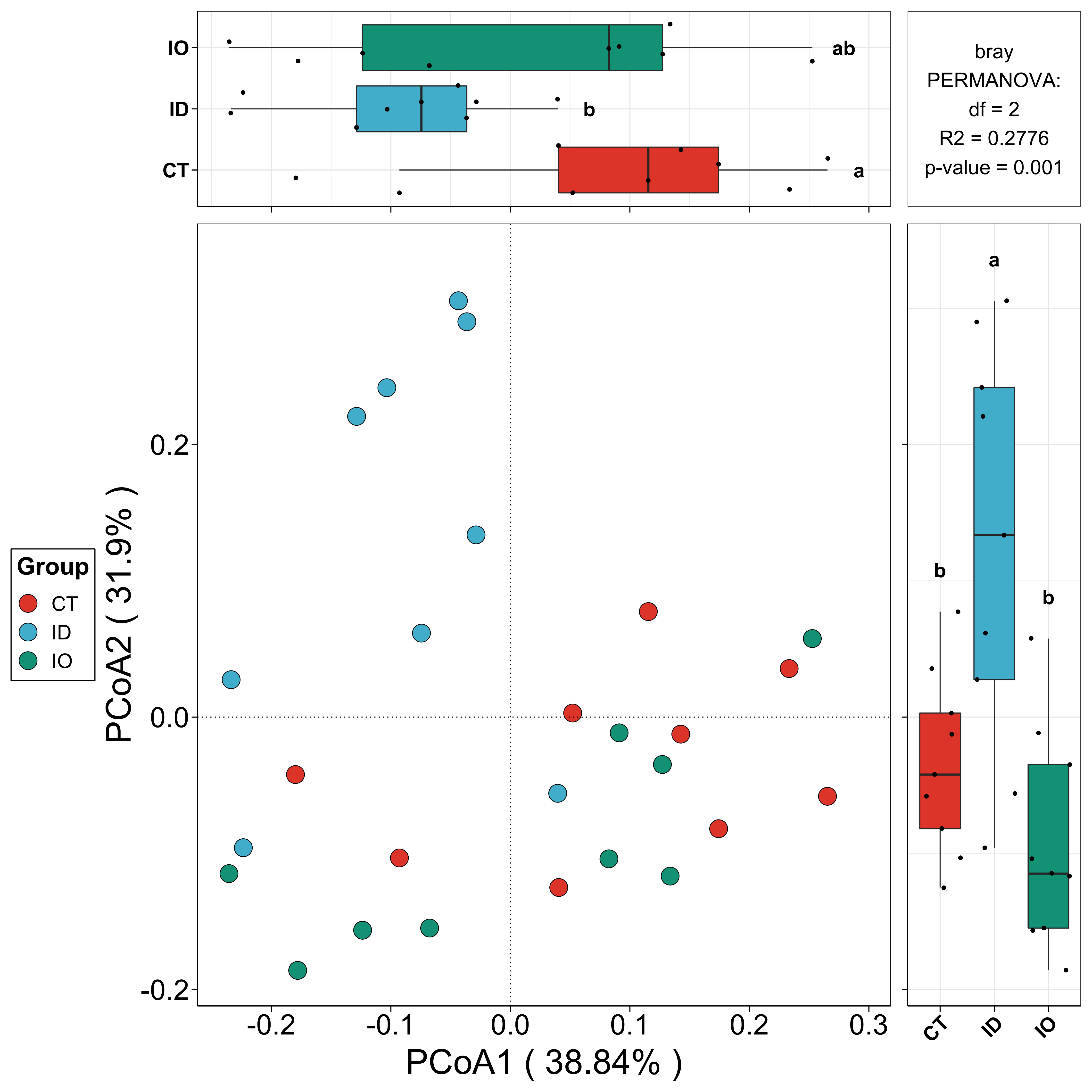
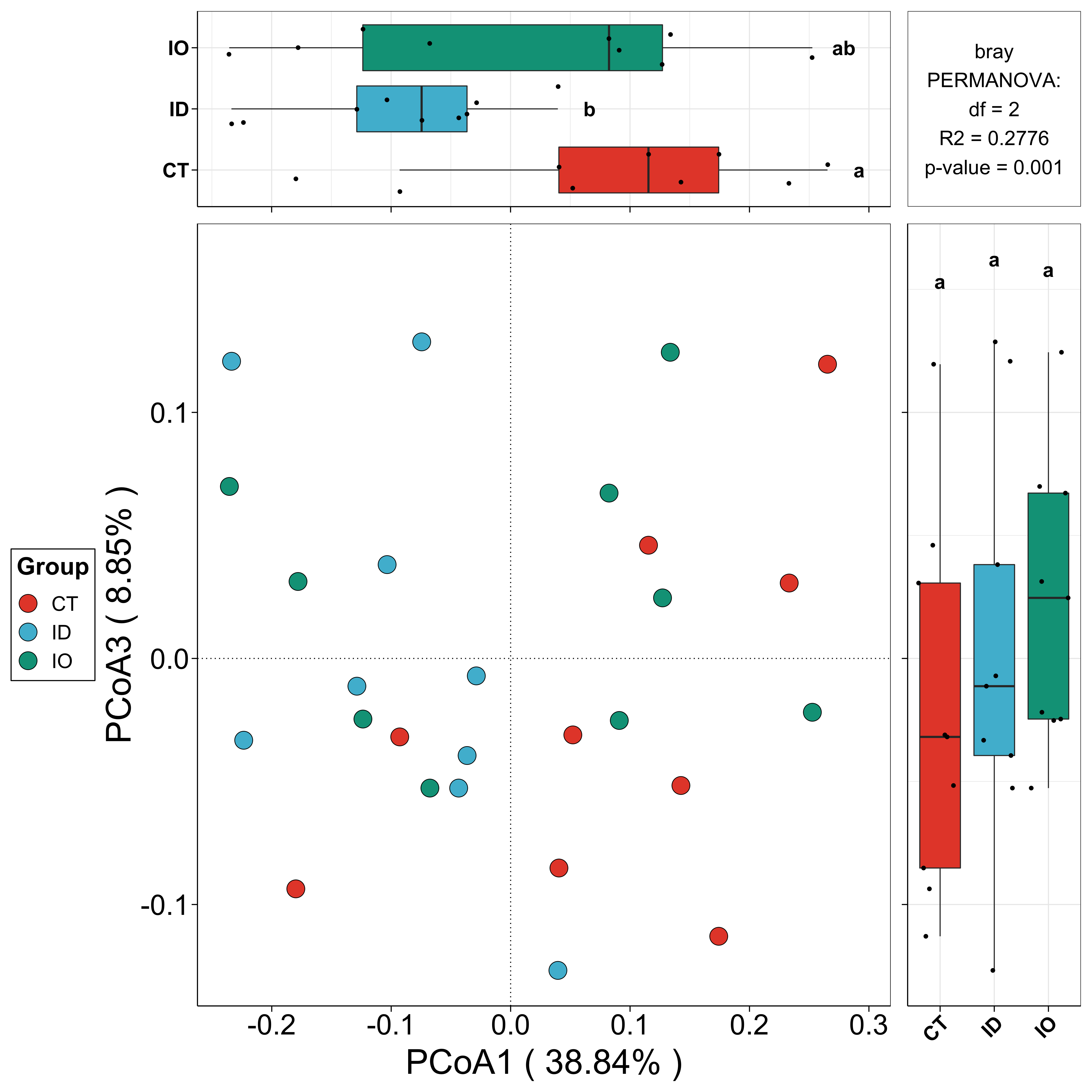
## Result
beta_re <- beta_plot(data = EMP$micro,design = EMP$mapping,min_relative = 0.001,min_ratio = 0.7,distance = 'bray')
## Plot
beta_re$plot$species$pic$p12
## Interactive visualization
beta_re$plot$species$html$p12

## Load data
data(EMP)

## Result
## When ** cooc_output = T **, cooc picture is generated in working directory.
 cooc_re <- cooc_plot(data = EMP$micro,design = EMP$mapping,min_relative = 0.001,min_ratio = 0.7,cooc_method = 'spearman',cooc_output = T)
##show attributes of net analysis profile at different levels
 cooc_re$cooc_profile$species


## If some globe parameters do not works well for specific plot,
## ** cooc_plot_each ** is prepared for this.
 cooc_plot_each(result$plot$Control$species,cooc_output=T,vertex.size = 8,
 	   vertex.label.cex =2 ,edge.width =2 )

## Load data
 library(EasyMicroPlot)
 data(EMP)


## Generate Top abundance barplot (easy running in default parameters)
 structure_re <- structure_plot(data = EMP$micro,design = EMP$mapping,
                                 min_relative = 0.001,min_ratio = 0.7)

## Plot
 structure_re$pic$genus$barplot$Total
 structure_re$pic$genus$barplot$CT


## Show top abundance taxonomy
 structure_re$result$filter_data$species
 structure_re$result$filter_data$species_ID


## Support ggplot theme parameters
 library(ggplot2)
 newtheme_slope=theme(axis.text.x =element_text(angle = 45, hjust = 1,size = 10))
 structure_re <- structure_plot(data = EMP$micro,design = EMP$mapping,
                               min_relative = 0.001,min_ratio = 0.7,mytheme =newtheme_slope)
 structure_re$pic$family$barplot$Total

## Load data
library(EasyMicroPlot)
data(EMP)
## Data preparation
core_data <- data_filter(data = EMP$micro,design = EMP$mapping,
min_relative = 0.001,min_ratio = 0.7)
sp <- core_data$filter_data$species
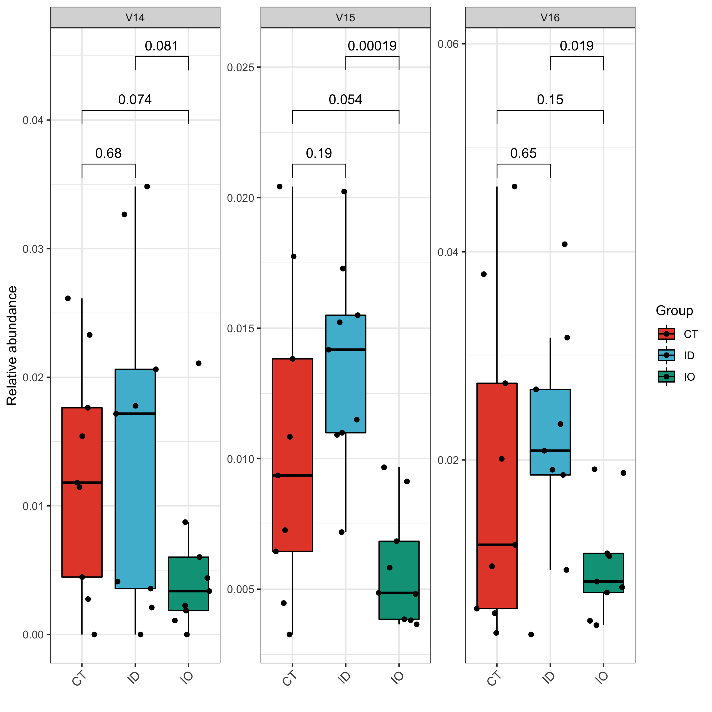
## Taxonomy boxplot
## For Student-Test in comparation
tax_re <- tax_plot(data = sp,tax_select = c('V14','V15','V16'),method = 'ttest')
## For one-way ANOVA and Post Hoc test
tax_re <- tax_plot(data = sp,tax_select = c('V14','V15','V16'),method = 'SNK')
## Plot
tax_re$pic$V14
## Interactive visualization
tax_re$html$V14
## Support ggplot theme parameters
library(ggplot2)
newtheme_slope=theme(axis.text.x =element_text(angle = 45, hjust = 1,size = 10))
tax_re <- tax_plot(data = sp,tax_select = c('V14','V15','V16'),method = 'ttest',mytheme = newtheme_slope)

## Load data
 library(EasyMicroPlot)
 data(EMP)

## Generate core data
 core_data <- data_filter(data = EMP$micro,design = EMP$mapping,
                             min_relative = 0.001,min_ratio = 0.7)
## Prepare training data
 sp <- core_data$filter_data$species

## Generate rfcv
 RFCV_result <- RFCV(sp)

## Show RFCV curve
 RFCV_result$RFCV_result_plot$curve_plot

## Show intersection and union tax among all the best models under different random number seed
 RFCV_result$RFCV_result_plot$intersect_num
 RFCV_result$RFCV_result_plot$union_num

## Load data
 library(EasyMicroPlot)
 data(EMP)

## Generate core data
 core_data <- data_filter(data = EMP$micro,design = EMP$mapping,
                             min_relative = 0.001,min_ratio = 0.7)
## Prepare training data
 sp <- core_data$filter_data$species

## Modify the group into two cases when multiple group exists.
 sp <- RFCV_data_binary(sp,rf_estimate_group = 'ID',id_not = 'NO_ID')
## Load data
 library(EasyMicroPlot)
 data(EMP)

## Generate core data
 core_data <- data_filter(data = EMP$micro,design = EMP$mapping,
                             min_relative = 0.001,min_ratio = 0.7)
## Prepare training data
 sp <- core_data$filter_data$species

## Modify the group into two cases when multiple groups exist.
 sp <- RFCV_data_binary(sp,rf_estimate_group = 'CT',id_not = 'Cases')

## Generate rfcv
 RFCV_result <- RFCV(sp)

## Show intersection and union tax among all the best models under different random number seed
 RFCV_result$RFCV_result_plot$intersect_num
 RFCV_result$RFCV_result_plot$union_num

## ROC
## Parameter *rf_tax_select* allows users to select optional tax
## **union** and **intersect** means the intersection and union tax of models above
RFCV_roc(RFCV_result,rf_tax_select = c("V143", "V83" , "V101", "V121"),rf_estimate_group = 'Cases')
RFCV_roc(RFCV_result,rf_tax_select = 'union',rf_estimate_group = 'Cases')
RFCV_roc(RFCV_result,rf_tax_select = 'intersect',rf_estimate_group = 'Cases')

## Load data
library(EasyMicroPlot)
data(EMP)
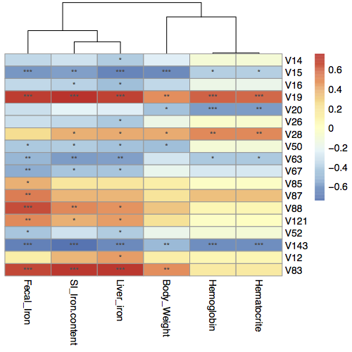
## Prepare the bacteria taxa data
core_data <- data_filter(data = EMP$micro,design = EMP$mapping,
min_relative = 0.001,min_ratio = 0.7)
sp <- core_data$filter_data$species
## Analysis and plot
## When ** cor_output = T **, cooc picture is generated in working directory.
cor_re <- EMP_COR(data = sp,meta=EMP$iron,cor_output = T,method = 'spearman',aes_value = 1)
cor_re <- EMP_COR(data = sp,meta=EMP$iron,cor_output = T,method = 'spearman',aes_value = 2)